Introduction

For accurate fitting of muscle diffusion tensor imaging data, many methods have been proposed. Linear solvers that account for data outliers, i.e. REKINDLE (1), and iterative reweighted linear least squares are commonly recommended (2,3). Additionally, to account for muscle perfusion IVIM correction of the diffusion data was proposed (4). Although linear solvers are fast the iterative reweighting slows down the fitting. Additionally, combining the DTI model with IVIM prevents the use of linear solvers. To circumvent this one can first fit the IVIM model and then fix the perfusion components allowing for a Linear solution to the DTI model. Recently, promising alternative solutions using neural nets for IVIM fitting were introduced (5,6). In this study, the performance of an unsupervised physics-informed deep learning method for combined IVIM and DTI fitting of muscle DTI data is investigated.

Methods

DWI data of the thighs of 20 subjects (10 male 10 female) was used. All MR examinations were performed on a 3 T MR scanner (Philips Ingenia, Philips Medical Systems, the Netherlands). Subjects were scanned in the supine position, feet-first with a 12-channel posterior and 16-channel anterior body coil, and field of view (FOV) set at 17.5 cm distance from the upper limit of the femoral head stretching 15 cm towards the knee. The spin-echo EPI DWI acquisition comprised 8 b-values (0 (1), 1 (6), 10 (3), 25 (3), 100 (3), 200 (6), 400 (8), 600 (12)) with 42 total acquisitions. Acquisition parameters were: TR = 5000ms; TE = 57 ms; resolution 3x3x6 mm³; Acquisition matrix = 160x92; Number of slices = 25; SENSE = 1.9; Partial Fourier = 0.75; and triple fat suppression by Gradient inversion + SPAIR (main fat signal) + SPIR (olefinic fat signal) 1.9/0.75, with a total acquisition time of 3min30s.
Data processing and fitting were performed using QMRITools for Mathematica (github.com/mfroeling/QMRITools). Data were preprocessed using PCA denoising for noise reduction and affine registration to correct for subject motion and eddy current deformations (7). Next data were fitted using a traditional iWLLS algorithm with IVIM correction (NLS) and using a self-learning physics informed neural net (NN).
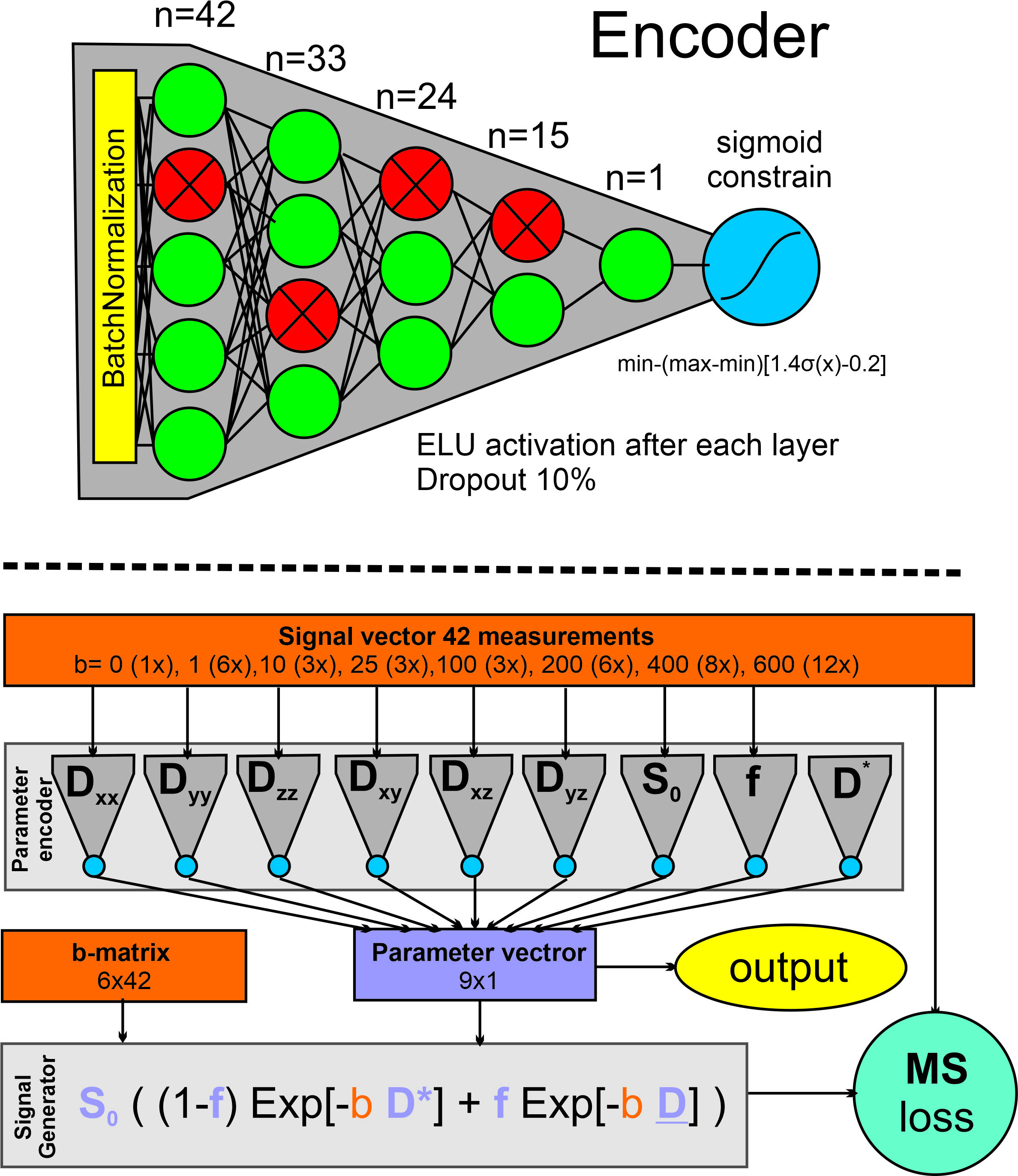
The neural net comprised 9 fully connected networks (4 layers deep), one for each parameter see Figure 1. Before each network batch-normalization was performed and during training, a dropout rate of 10% was used. The resulting parameter vector obtained by the NN was fed to a signal generator using the combined IVIM and DTI equations. The net loss was defined as the mean square error between the data and the generated signal. The network was trained using an ADAM optimizer with a learning rate of 10-4. To train the network 20.000 voxels were randomly selected from all datasets. The training was done with a batch size of 64 for 15 epochs using an NVidia Quadro M1000 GPU with 2 Gb ram.
After fitting mean muscle values for the derived parameters were calculated for 12 muscles in each leg, i.e. Sartorius, Rectus Femoris, Vastuslateralis, Vastus Intermedius, Vastus Medialis, Biceps Femoris Long head, Semitendinosus, Semimembranosus, Gracilis, Adductor Longus, Adductor Magnus, Biceps Femoris Short head.

Results

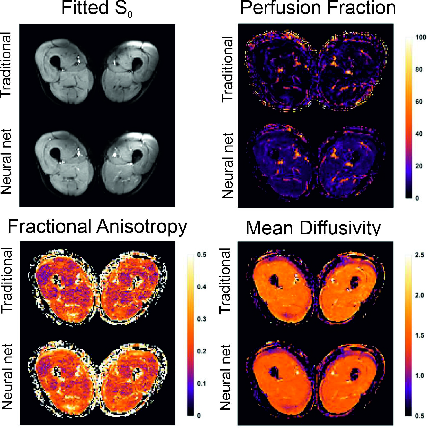
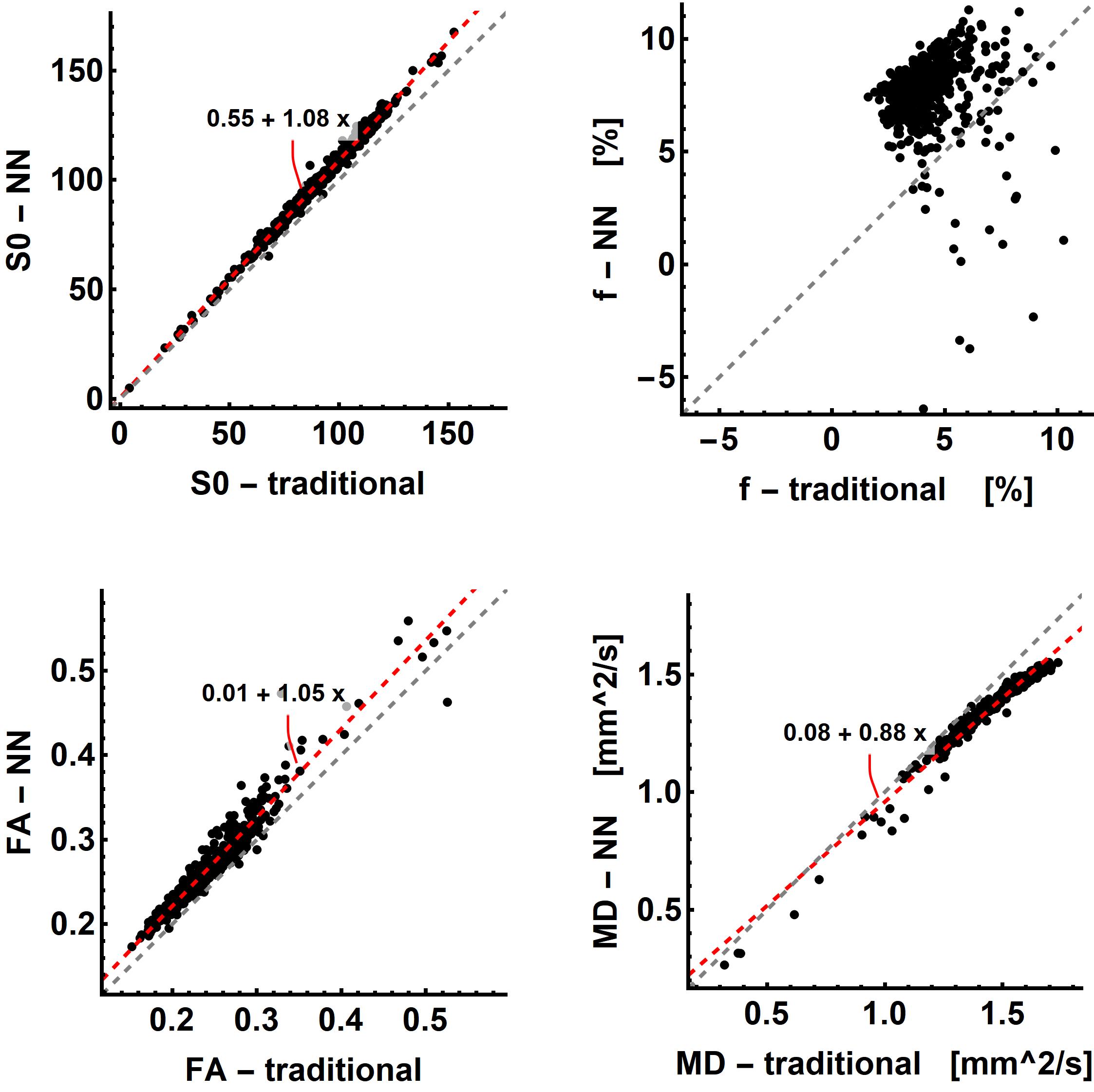
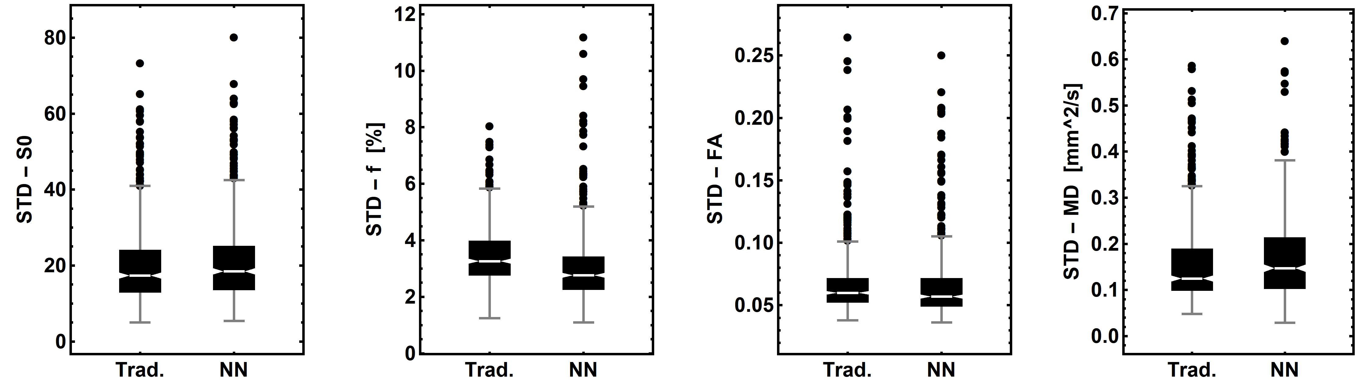
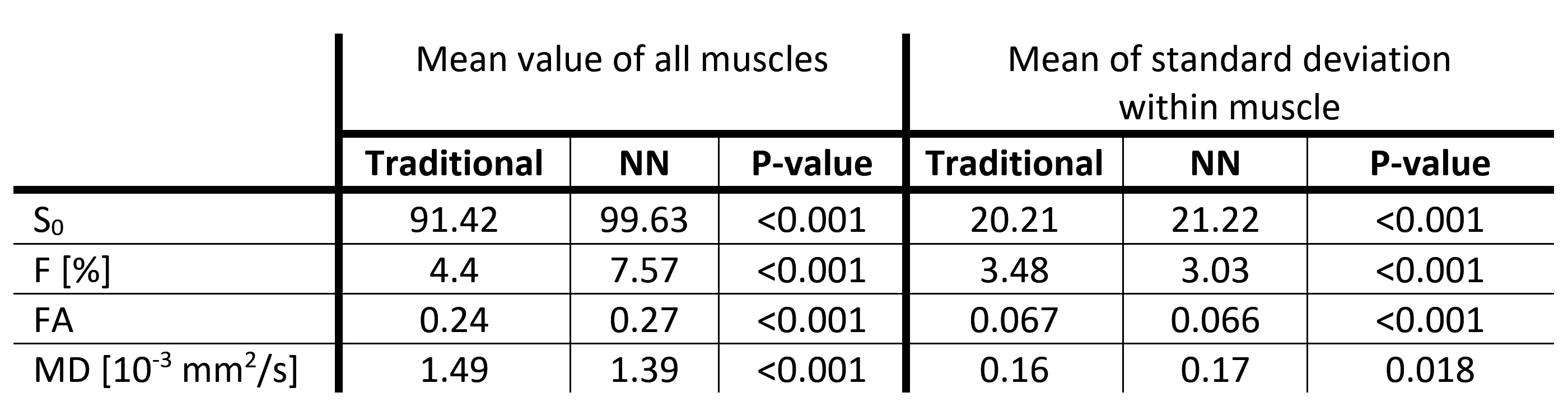
The neural net trained in 45s and fitting a full dataset took around 4s. The traditional processing took around 10min per dataset. The parameter maps of the traditional and NN fitting are shown in figure 2 and both look similar. The most apparent difference is the increased signal fraction of the IVIM components when fitting with the NN. As a result, the MD is decreased and the FA is increased since the IVIM component is an isotopic one as can be seen in figure 3. Furthermore, the standard deviation of the estimated parameters within each muscle was comparable as is shown in figure 4. However, although all parameters and variations appear similar statistical testing (signed-rank test) showed that all differences were significant as is shown in table 1.

Discussion and Conclusion

We have shown that a self-learning physics informed neural net is capable of fitting the combined IVIM-DTI model within seconds per dataset. Such accelerated fitting will allow for better clinical translation of muscle DTI since currently slow offline processing is needed. Although differences between the traditional and NN fitting are small they are significant. Further investigation is needed to understand the origins of these differences. In conclusion, fast and robust fitting of muscle DTI data is feasible using neural nets.

Acknowledgements

No acknowledgement found.