0806
DeepPain: Uncovering Associations Between Data-Driven Learned qMRI Biomarkers and Chronic Pain
Alejandro Morales Martinez1, Jinhee Lee1, Francesco Caliva1, Claudia Iriondo1, Sarthak Kamat1, Sharmila Majumdar1, and Valentina Pedoia1
1UCSF, San Francisco, CA, United States
1UCSF, San Francisco, CA, United States
Synopsis
Large-scale analysis of the relationship between learned qMRI biomarkers and chronic knee pain. 7,437 patient timepoints reporting chronic pain were used to train three different deep learning models for bone shape, cartilage thickness, and cartilage T2 biomarkers for the femur, tibia, and patella. The true chronic knee pain predictions for each trained model were further investigated with Grad-CAM and the max activation values for each model were sorted into clinically relevant anatomical compartments for each bone. Bone shape and cartilage T2 seemed to be spatially correlated based on the results of the analysis.
Introduction
Osteoarthritis (OA) is a degenerative joint disease characterized by the gradual deterioration of cartilage, bone and synovium. The lack of noninvasive treatment options to reverse the progression of structural joint degeneration has shifted the medical care of knee OA to symptomatic pain management in a clinical setting1,2. While there is a widely perceived association of structural change with pain, previous studies linking radiographic OA to the presence of knee pain have not yet verified a strong correlation3,4. Leveraging the superior soft tissue contrast of MRI over radiographs to monitor the soft tissue changes thought to be related with knee pain could better our understanding of symptomatic OA. This study aims to uncover latent relationships between chronic knee pain and imaging biomarkers by exploring the ability of deep learning convolutional neural networks to use morphological and compositional features of the femur, tibia, and patella to diagnose chronic knee pain.Methods
The Osteoarthritis Initiative (OAI) dataset5 used for this study contains 3D double-echo steady-state (3D-DESS, 3T Siemens, TR/TE 16.2/4.7; FOV, 14 cm; matrix, 307x384; bandwidth, 71 kHz; and image resolution, [0.365, 0.456, 0.7] mm) and 2D multi-slice multi-echo (2D-MSME, 3T Siemens, TR/TE 2700/10,20,30,40,50,60,70; FOV, 12 cm; matrix, 269x384; bandwidth, 96 kHz; and image resolution, [0.313, 0.446, 3] mm) MRI knee scans from a total of 4,796 unique patients for 12 different time points for both knees. Overall processing pipeline is shown in Figure 1. A bone and a cartilage segmentation model ensemble were trained on 72 and 148 manually segmented 3D-DESS volumes to segment the femur, tibia, and patella bones and corresponding cartilage6. The trained models were used to segment 7,437 3D-DESS volumes (Figure 1A). Bone shape7 and cartilage thickness maps were obtained from the segmented masks. T2 values were calculated by registering 3D-DESS cartilage masks to the matching MSME MRI volumes and performing parametric T2 fitting on the cartilage. Each biomarker was projected onto the articular bone surface (Figure 1B) and transformed into spherical coordinates (Figure 2). Three different strategies were performed to merge spherical maps for each bone (Figure 3). A total of 7,437 merged spherical maps with corresponding chronic pain labels were used to train ResNet508 binary classifier models to diagnose chronic knee pain using each merging strategy (Figure 1D). Chronic knee pain was defined as patient timepoints which reported knee pain, aching, or stiffness over half of the days of the month for more than six months of the past 12 months. The true positive test set cases for each trained model were analyzed using Grad-CAM9 maps from the last convolutional layer of each model. The max Grad-CAM activation for each model was recorded and assigned into clinically relevant anatomical compartments for each bone. The compartments for the femur were medial, anterior, lateral, medial posterior, and lateral posterior. The compartments for the tibia were medial anterior, medial posterior, lateral anterior, and lateral posterior. The compartments for the patella were medial distal, medial proximal, lateral distal, and lateral proximal. The chronic pain diagnosis dataset included a total of 7,437 MRI scans (4,989 (67%) no pain and 2,448 (33%) chronic pain) split into 4,438/910/2,089 sets for the training, validation and test sets respectively. The demographics distribution, such as age, body mass index (BMI), and sex with corresponding 95% confidence interval (CI95) for the 7,437 patients was 63.9 ± 0.2, 28.2 ± 0.1 and 3,510/3,927 male/female respectively.Results
The bone segmentation mean test dice scores with corresponding CI95 were 98.0% ± 0.3%, 98.0% ± 0.3%, and 96.4% ± 0.7% for the femur, tibia, and patella respectively. The cartilage segmentation mean test dice scores with corresponding CI95 were 90.0% ± 0.7%, 88.6% ± 1.3%, and 85.7% ± 2.5% for the femoral, tibial, and patellar cartilage respectively. The test sensitivity/specificity/area under the curve (AUC) with corresponding CI95 for the femur chronic pain models were 49.6 ± 0.4/83.4 ± 0.2/72.7 ± 0.242, 45.2 ± 0.4/85.6 ± 0.2/69.7 ± 0.3, and 51.6 ± 0.3/76.6 ± 0.2/70.0 ± 0.3 for the bone shape, cartilage thickness and cartilage T2 models respectively. The test sensitivity/specificity/AUC with corresponding CI95 for the tibia chronic pain models were 51.4 ± 0.4/76.5 ± 0.2/69.6 ± 0.2, 50.6 ± 0.3/75.8 ± 0.2/67.7 ± 0.2, and 46.8 ± 0.3/76.8 ± 0.2/65.6 ± 0.2 for the bone shape, cartilage thickness and cartilage T2 models respectively. The test sensitivity/specificity/AUC with corresponding CI95 for the patella chronic pain models were 67.3 ± 0.3/56.8 ± 0.3/68.3 ± 0.2, 52.4 ± 0.4/73.4 ± 0.2/69.6 ± 0.3, and 52.1 ± 0.4/75.6 ± 0.3/68.3 ± 0.2 for the bone shape, cartilage thickness and cartilage T2 models respectively. The results of the Grad-CAM analysis are shown on Figure 4 and Figure 5.Discussion and Conclusion
The findings suggest that there is a spatial correlation between bone shape and cartilage T2 when it comes to predicting whether a patient is exhibiting chronic pain. Additionally, the activations are quite varied across each bone, pointing to a multifactorial combination of biomarkers behind chronic knee pain. With this study, we have leveraged deep learning architectures and the multimodal nature of MRI to discover new associations between chronic knee pain and quantitative imaging biomarkers.Acknowledgements
NIAMS Grants:
- R00AR070902
- R61AR073552
References
- Bhosale AM, Richardson JB. Articular cartilage: structure, injuries and review of management. Br Med Bull. 2008;87(1):77-95. doi:10.1093/bmb/ldn025
- Goodwin DW, Dunn JF. High-Resolution Magnetic Resonance Imaging of Articular Cartilage: Correlation with Histology and Pathology. Top Magn Reson Imaging. 1998;9(6):337.
- Minciullo L, Parkes MJ, Felson DT, Cootes TF. Comparing image analysis approaches versus expert readers: the relation of knee radiograph features to knee pain. Ann Rheum Dis. 2018;77(11):1606-1609. doi:10.1136/annrheumdis-2018-213492
- Neogi T, Frey-Law L, Scholz J, et al. Sensitivity and sensitisation in relation to pain severity in knee osteoarthritis: trait or state? Ann Rheum Dis. 2015;74(4):682-688. doi:10.1136/annrheumdis-2013-204191
- Peterfy CG, Schneider E, Nevitt M. The osteoarthritis initiative: report on the design rationale for the magnetic resonance imaging protocol for the knee. Osteoarthr Cartil OARS Osteoarthr Res Soc. 2008;16(12):1433-1441. doi:10.1016/j.joca.2008.06.016
- Iriondo C, Liu F, Calivà F, Kamat S, Majumdar S, Pedoia V. Towards Understanding Mechanistic Subgroups of Osteoarthritis: 8 Year Cartilage Thickness Trajectory Analysis. J Orthop Res. n/a(n/a). doi:10.1002/jor.24849
- Martinez AM, Caliva F, Flament I, et al. Learning osteoarthritis imaging biomarkers from bone surface spherical encoding. Magn Reson Med. n/a(n/a). doi:10.1002/mrm.28251
- He K, Zhang X, Ren S, Sun J. Deep Residual Learning for Image Recognition. ArXiv151203385 Cs. Published online December 10, 2015. Accessed November 6, 2018. http://arxiv.org/abs/1512.03385
- Selvaraju RR, Cogswell M, Das A, Vedantam R, Parikh D, Batra D. Grad-CAM: Visual Explanations from Deep Networks via Gradient-based Localization. ArXiv161002391 Cs. Published online October 7, 2016. Accessed May 13, 2019. http://arxiv.org/abs/1610.02391
Figures
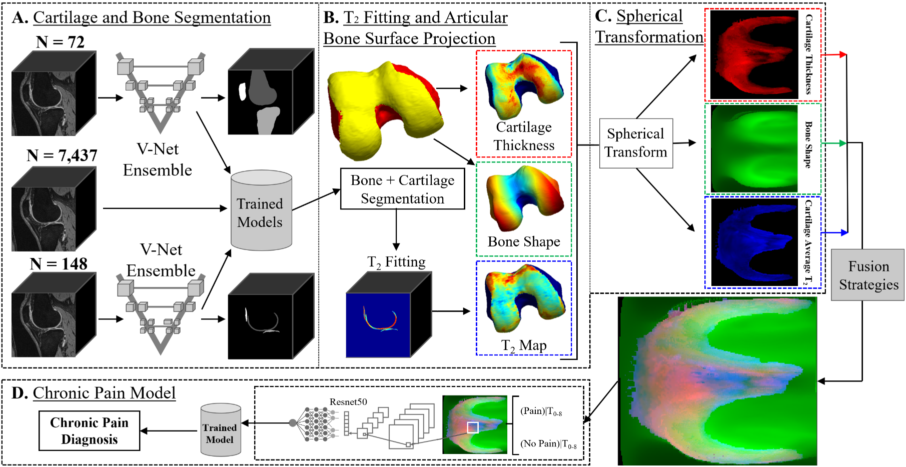
Overview of the pipeline. (A) A bone and a cartilage
segmentation model ensemble were trained on manually segmented 3D-DESS and used to segment bone and cartilage from 7,437 3D-DESS. (B)
Bone shape and cartilage thickness maps were obtained from segmentations. Cartilage T2 values were parametrically fitted after registering 3D-DESS
cartilage to matching MSME. Each biomarker was projected onto the articular bone surface and transformed into spherical coordinates (C). (D) The merged spherical maps were used to
train classifier models to diagnose chronic knee pain.
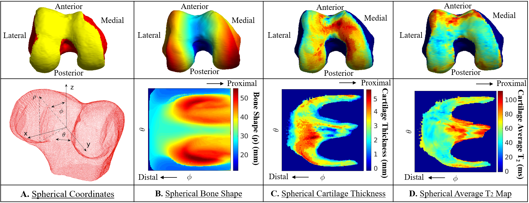
Femur spherical maps. (A) The transformation from Cartesian coordinates into spherical coordinates was performed by
uniformly sampling 224 x 224 points in the point cloud and describing them
based on the angle along the x-y plane from the positive x-axis (θ), the
elevation angle from the x-y plane (φ) and the distance from the center of the
point cloud to the sampled point in the surface (ρ). The sampling was
designed to be centered around the articular surface. (B) Bone shape 2D spherical map. (C) Cartilage
thickness 2D spherical map. (D) Cartilage average T2 value 2D
spherical map.
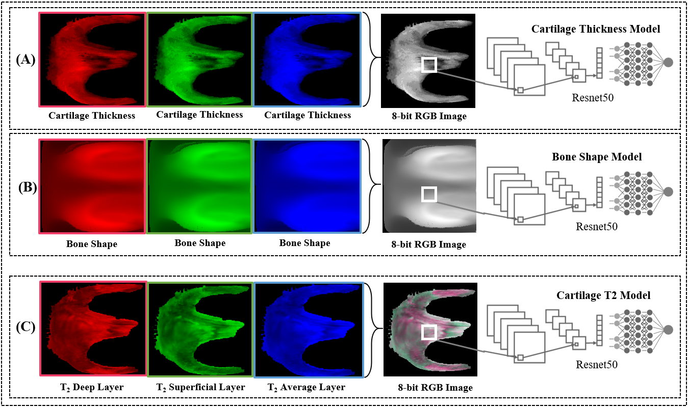
Overview of the biomarker model strategies, shown for the
femur. The group normalized spherical images for each patient were merged into
a three-channel 8-bit image. (A) The cartilage thickness strategy consisted of
the cartilage thickness spherical maps replicated three times into a spherical
image. (B) The bone shape strategy consisted of the bone shape spherical maps
replicated three times into a spherical image. (C) The cartilage T2 strategy consisted of the deep, superficial, and
average T2 spherical maps as the first, second, and
third channels respectively.
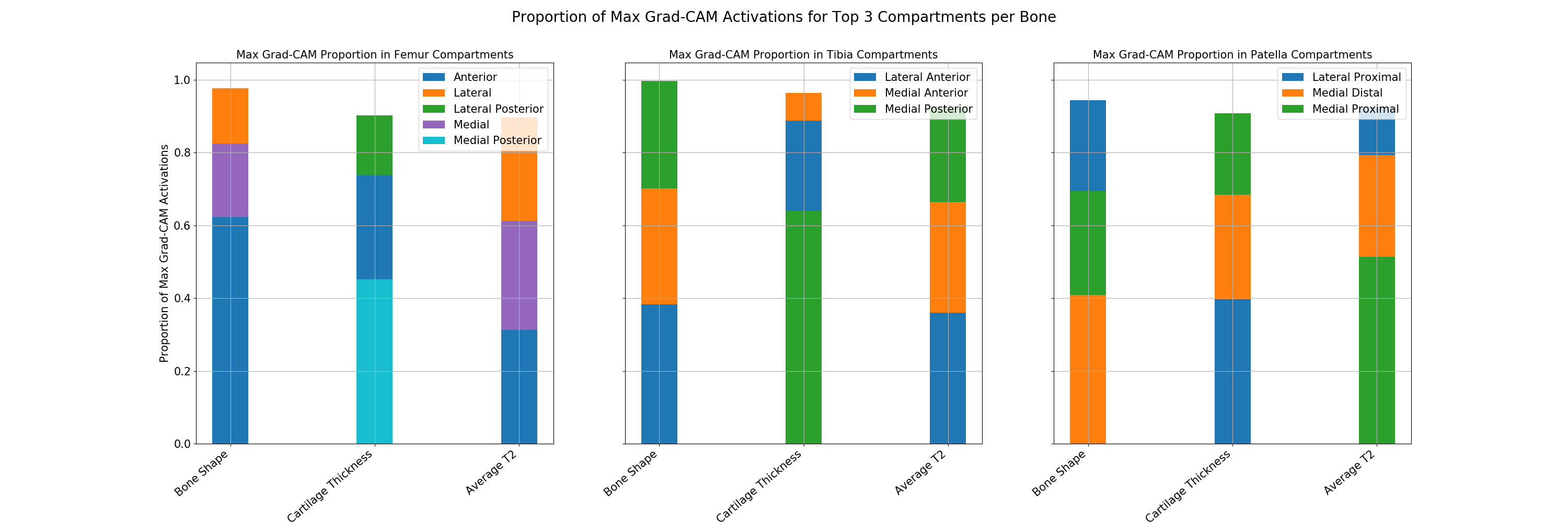
Results of the Grad-CAM analysis for each model. The Grad-CAM activation maps were calculated by combining the feature maps from the last convolutional layer of each model. The max activation value for each model was categorized into clinically relevant anatomical compartments for each bone. The compartments were medial, anterior, lateral, medial posterior,
and lateral posterior for the femur, medial anterior, medial
posterior, lateral anterior, and lateral posterior for the tibia, and medial distal, medial proximal, lateral distal, and lateral proximal for the patella.
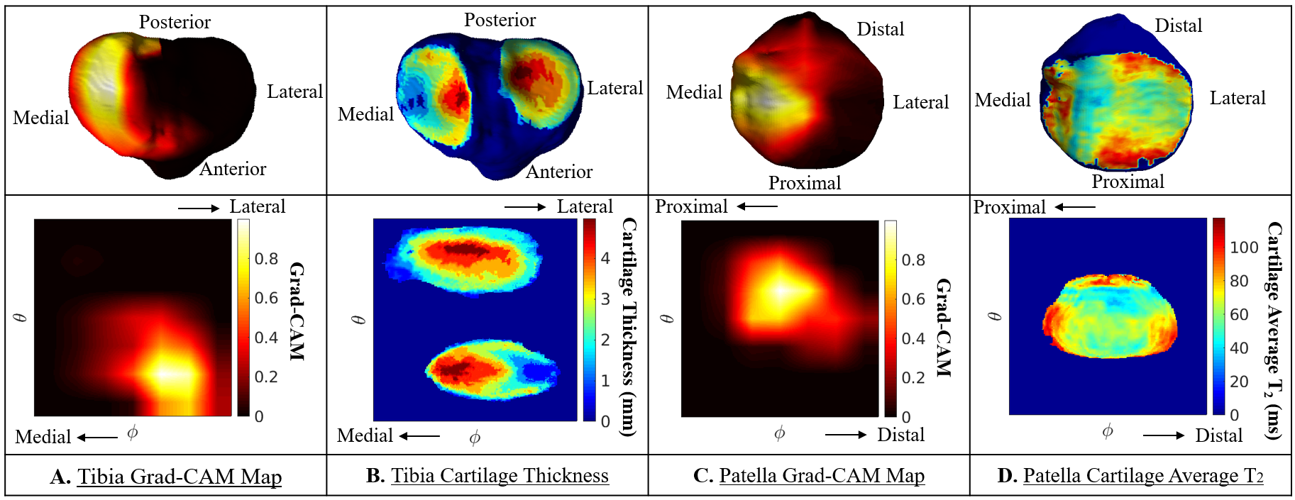
Grad-CAM activation spherical maps overlaid on the articular bone surface for the tibia and patella cartilage thickness and cartilage T2 models respectively. (A) Tibia Grad-CAM spherical map and projection shows a high activation in the medial tibia. (B) Same tibia cartilage thickness spherical map and projection shows cartilage thinning in the medial tibial cartilage. (C) Patella Grad-CAM spherical map and projection shows a high activation in the medial patella. (D) Same patella cartilage T2 spherical map and projection shows elevated T2 values in the medial patellar cartilage.