0790
Decompose QSM to diamagnetic and paramagnetic components via a complex signal mixture model of gradient-echo MRI data1Department of Electrical Engineering and Computer Sciences, University of California, Berkeley, Berkeley, CA, United States, 2Vector Lab for Intelligent Medical Imaging and Neural Engineering, International Innovation Center of Tsinghua University, Shanghai, China, 3Helen Wills Neuroscience Institute, University of California, Berkeley, Berkeley, CA, United States
Synopsis
We propose and develop a method to separate paramagnetic and diamagnetic components within one voxel based on a 3-pool signal model. Alternating between solving for linear and nonlinear parameters in the model, paramagnetic component susceptibility (PCS) and diamagnetic component susceptibility (DCS) maps are constructed to represent the sub-voxel compartments.
INTRODUCTION
Quantitative Susceptibility Mapping (QSM) has been shown potential utilities for imaging a number of diseases including PD1,2 and MS3,4 as well as for investigating normal brain structures5,6. QSM, however, does not characterize the sub-voxel susceptibility distribution. With the current resolution of MRI, one voxel may contain both paramagnetic and diamagnetic susceptibility sources. If equal amount of paramagnetic and diamagnetic susceptibility exists in one voxel, the total QSM would appear to be zero. There have been a few attempts to separate the opposing susceptivity sources7,8. Those models are based on the assumption that the mean QSM of one voxel is the linear summation of paramagnetic and diamagnetic components. However, the fundamental signal progression of a multi-echo gradient echo sequence (GRE) involves complex exponentials. Hereby, we develop a method to estimate the opposing susceptibility sources within a voxel using solely multi-echo GRE data by solving a complex nonlinear equation. We refer the method as DiamagnEtic COMponent and Paramagnetic cOmponent SEparation or DECOMPOSE-QSM.THEORY
DECOMPOSE-QSM is based on a 3-pool signal model.Signals are contributing from 3 components with corresponding volume susceptibility $$$\chi_+$$$, $$$\chi_-$$$, and $$$\chi_0$$$ ( $$$\chi_{+,-,0}$$$for short), and corresponding transvers relaxation rate $$$R_{2,+}^\ast$$$, $$$R_{2,-}^\ast$$$and $$$R_{2,0}^\ast$$$ ( $$$R_{2,+,-,0}^\ast$$$for short), respectively. Note that the neutral medium is assumed to have zero volume susceptibility, i.e. $$$\chi_0=0$$$ . $$$R_{2,+,-,0}^\ast$$$ is known to be linearly related to the volume susceptibility based on the theory at static dephasing regime9,10,$$R_{2,+,-}^\ast=R_2^\prime+R_2=\frac{2\pi}{9\sqrt{3}}\gamma B_0 |\chi_{+,-}| +R_2=a|\chi_{+,-}|+b\tag{1}$$where $$$a=\frac{2\pi}{9\sqrt{3}}\gamma B_0$$$ evaluating at 3T is 323.5 Hz/ppm. The source of the magnetic susceptibility is modeled as a uniformly magnetized sphere. The field of the interior of a sphere with uniformly distributed susceptibility $$$\chi$$$ magnetized by the $$$B_0$$$ field is$$B_{in}=\frac{2}{3}\mu_0M_0=\frac{2}{3}\chi B_0\tag{2}$$while the field outside such a sphere is equivalent to a dipole field. As long as the majority of the dipole field is within the voxel, the total field perturbation of the voxel will predominantly come from the interior of the sphere as the exterior fields cancel out due to the dipole field distribution.Under these assumptions, the signal model is given by$$\begin{align}S(t;C_+,C_-,C_0,\chi_+,\chi_-,R^*_{2,0})=&C_+e^{-(a\chi_++R^*_{2,0}+i\frac{2}{3}\chi_+\gamma B_0)t}\\&+C_-e^{-(-a\chi_-+R^*_{2,0}+i\frac{2}{3}\chi_-\gamma B_0)t}\\&+ C_0e^{-R^*_{2,0}t}\end{align}\tag{3}$$
METHODS
While developing the solver, the parameters are being partitioned into linear ($$$C_+,C_-,C_0$$$) , linear after taking logarithm ($$$R_{2,0}^\ast$$$) and nonlinear ($$$\chi_+,\chi_-$$$) categories and solved in an alternating fashion,$$\begin{align}\min\lVert&\log(S(t;C_+,C_-,C_0,\chi_+,\chi_-,R^*_{2,0})-\log(y(t))\rVert\\s.t.:&C_++C_-+C_0=1\\&R_{2,0}^\ast>0\\&0.5 > |\chi_+|, |\chi_-|>0 \end{align}\tag{4}$$where$$$y(t)$$$is a synthesized complex gradient echo signal combining echo-time-dependent QSM and magnitude as follows$$y(t)=M(t)e^{-i\phi_{in}t}=M(t)e^{-i\frac{2}{3}\chi(t)\gamma B_0t}\tag{5}$$Taking the logarithm of the signal provides stronger weighting towards the phase of the signal, which turns out to result in a better-behaved cost function. Since logarithm is a monotonic function within the feasible set, such a modification will not change the optimality.The results are presented as Paramagnetic Component susceptibility (PCS) and Diamagnetic Component Susceptibility (DCS) derived from the compartmental model. Specifically,$$\text{PCS (or DCS)}=\frac{\sum_t\measuredangle(C_{+or-}e^{-(a|\chi_{+or-}|+R^*_{2,0}+i\frac{2}{3}\chi_{+or-}\gamma B_0)t}+(C_0+C_{-,or +})e^{-R^*_{2,0}t})}{\frac{2}{3}\gamma B_0\sum t}\tag{6}$$Likewise, the composite susceptibility map is then defined as$$\text{Composite susceptibility}=\frac{\sum_t\measuredangle((C_+e^{-(a|\chi_+|+i\frac{2}{3}\chi_+\gamma B_0)t}+C_+e^{-(a|\chi_-|+i\frac{2}{3}\chi_-\gamma B_0)t}+C_0)e^{-R^*_{2,0}t})}{\frac{2}{3}\gamma B_0\sum t}\tag{7}$$
RESULTS
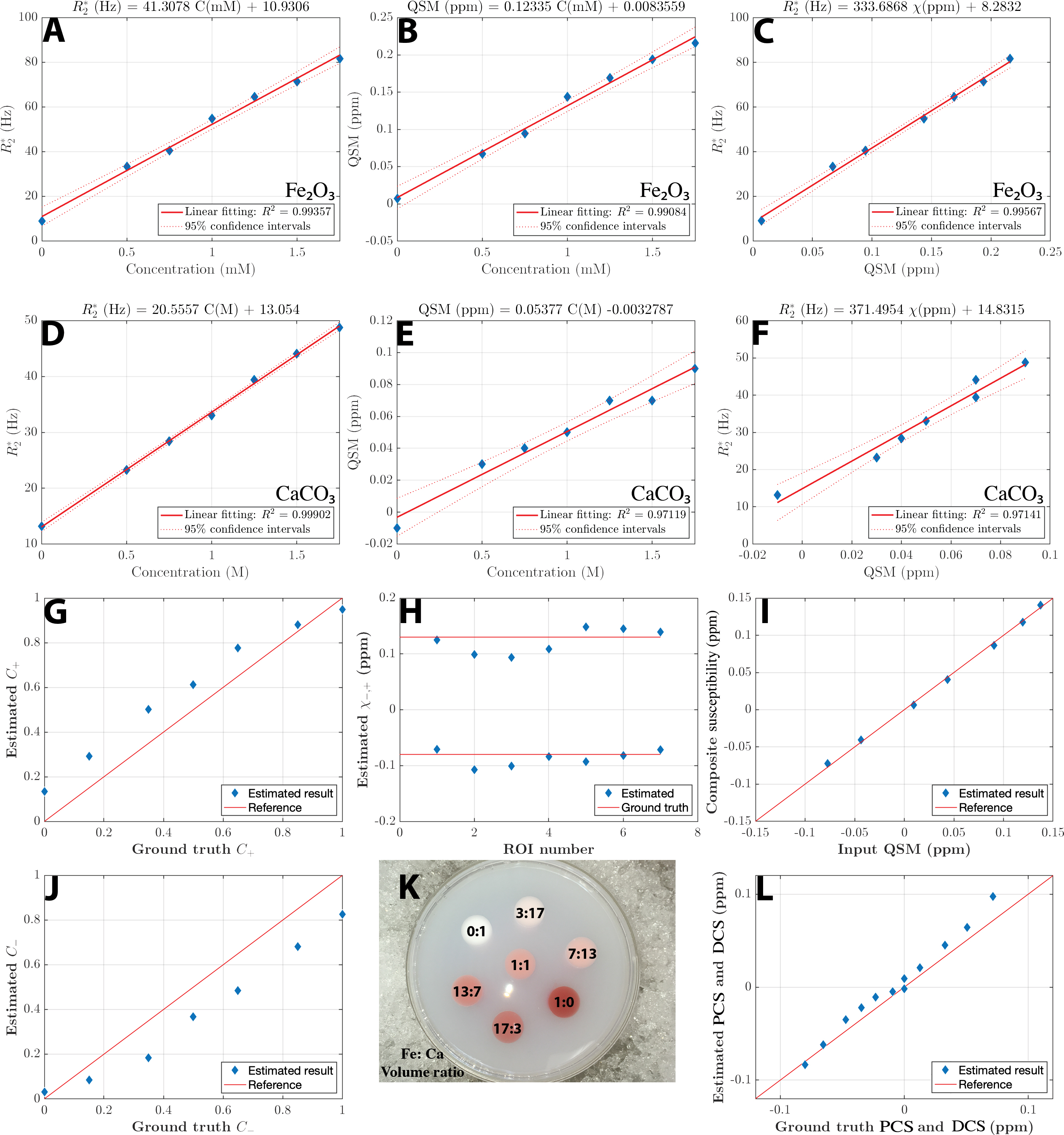
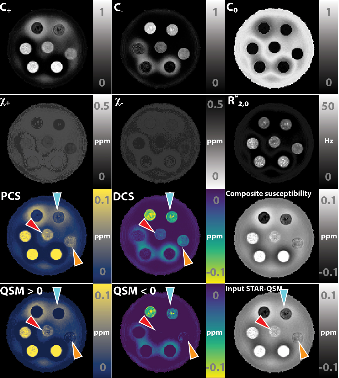
Simulation shows that the magnitude of mixture model remains largely exponential as a function of TE, while the phase develops a nonlinear TE dependency (Figure. 2B), consistent with previous report of TE-dependent QSM in the brain11. These results demonstrate that 1) it is necessary to use TE-dependent QSM as the input, and 2) phase information needs to play a significant role in the objective function to alleviate the difficulty of separating the summation of exponentials. In general, linear parameters showed a higher accuracy in estimation.Figure 3,4 show that susceptibilities of the phantom are separated into the PCS and DCS maps. The linear slope of $$$R_{2,+,-}\propto|\chi_{+,-}|$$$ was estimated to be 335 Hz/ppm for Fe2O3 phantom and 371 Hz/ppm for CaCO3 phantom. These values agree well with the theoretical estimation of 323.5 Hz/ppm. These results also agree with the reported fitting results (366 Hz/ppm) in the literature12 where 7T high-resolution images followed by COSMOS QSM calculation was carried out. In addition, the composite susceptibility agrees well the input QSM, demonstrating that DECOMPOSE-QSM does not alter the total volume susceptibility value.
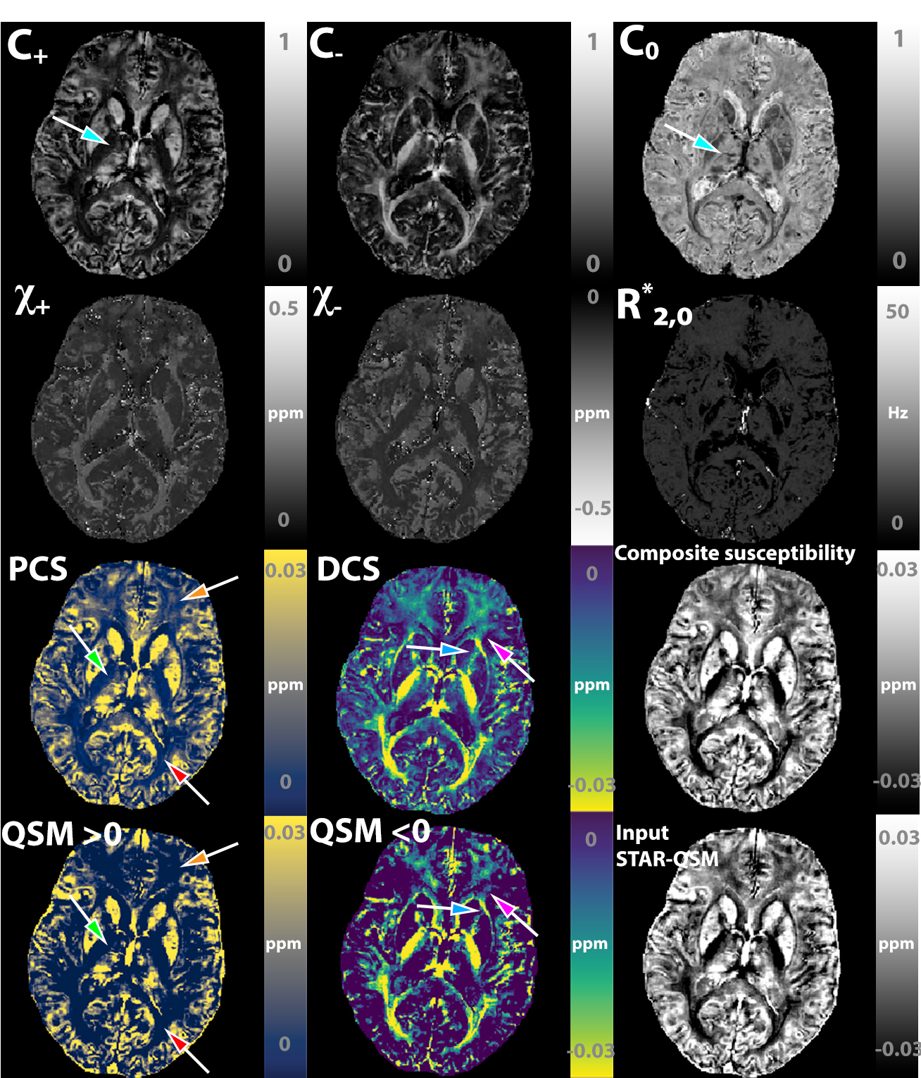
Figure 5 shows one representative case of the proposed algorithm being applied to a healthy subject’s brain. The PCS and DCS align with the known distribution of para-/dia-magenetic species in human cerebral region. Interestingly, the $$$C_0,C_+$$$ map reveals distinctive structural boundaries between subfields of thalamus, reflecting a variation of free water space or concentration among the various brain structures.
DISCUSSION
The proposed DECOMPOSE-QSM algorithm utilizes both the phase and magnitude information to separate susceptibility components within a voxel. The model consists of three pools of susceptibility sources that are spatially distributed: zero susceptibility (neutral or reference susceptibility), diamagnetic and paramagnetic susceptibility. The validity of the model was extensively tested and confirmed with numerical simulations. We further engineered a novel cost function and developed an effective optimization routine to solve this challenging nonlinear inverse problem. The accuracy of the solutions was demonstrated with extensive simulation, phantom experiments and in vivo brain scans. DECOMPOSE-QSM provides six parameters to characterize the susceptibility compartments: three volume fractions, two susceptibility values and one relaxation rate associated with the zero-susceptibility component. They are also combined to form PCS, DCS and composite susceptibility maps based on the complex signal model. We plan to further validate the method with independent measures and test its applications.Acknowledgements
No acknowledgement found.References
(1) Guan, X.; Huang, P.; Zeng, Q.; Liu, C.; Wei, H.; Xuan, M.; Gu, Q.; Xu, X.; Wang, N.; Yu, X.; Luo, X.; Zhang, M. Quantitative Susceptibility Mapping as a Biomarker for Evaluating White Matter Alterations in Parkinson’s Disease. Brain Imaging Behav 2019, 13 (1), 220–231. https://doi.org/10.1007/s11682-018-9842-z.
(2) He, N.; Ling, H.; Ding, B.; Huang, J.; Zhang, Y.; Zhang, Z.; Liu, C.; Chen, K.; Yan, F. Region-Specific Disturbed Iron Distribution in Early Idiopathic Parkinson’s Disease Measured by Quantitative Susceptibility Mapping. Human Brain Mapping 2015, 36 (11), 4407–4420. https://doi.org/10.1002/hbm.22928.
(3) Wisnieff, C.; Ramanan, S.; Olesik, J.; Gauthier, S.; Wang, Y.; Pitt, D. Quantitative Susceptibility Mapping (QSM) of White Matter Multiple Sclerosis Lesions: Interpreting Positive Susceptibility and the Presence of Iron. Magnetic Resonance in Medicine 2015, 74 (2), 564–570. https://doi.org/10.1002/mrm.25420.
(4) Zhang, Y.; Gauthier, S. A.; Gupta, A.; Comunale, J.; Chiang, G. C.-Y.; Zhou, D.; Chen, W.; Giambrone, A. E.; Zhu, W.; Wang, Y. Longitudinal Change in Magnetic Susceptibility of New Enhanced Multiple Sclerosis (MS) Lesions Measured on Serial Quantitative Susceptibility Mapping (QSM). Journal of Magnetic Resonance Imaging 2016, 44 (2), 426–432. https://doi.org/10.1002/jmri.25144.
(5) Wei, H.; Xie, L.; Dibb, R.; Li, W.; Decker, K.; Zhang, Y.; Johnson, G. A.; Liu, C. Imaging Whole-Brain Cytoarchitecture of Mouse with MRI-Based Quantitative Susceptibility Mapping. NeuroImage 2016, 137, 107–115. https://doi.org/10.1016/j.neuroimage.2016.05.033.
(6) Zhang, Y.; Wei, H.; Cronin, M. J.; He, N.; Yan, F.; Liu, C. Longitudinal Atlas for Normative Human Brain Development and Aging over the Lifespan Using Quantitative Susceptibility Mapping. NeuroImage 2018, 171, 176–189. https://doi.org/10.1016/j.neuroimage.2018.01.008.
(7) Lee, J.; Nam, Y.; Choi, J. Y.; Shin, H.; Hwang, T.; Lee, J. Separating Positive and Negative Susceptibility Sources in QSM. ISMRM, HONOLULU, HI, USA, MRM.[Google Scholar] 2017.
(8) Schweser, F.; Deistung, A.; Lehr, B.; Sommer, K.; Reichenbach, J. SEMI-TWInS: Simultaneous Extraction of Myelin and Iron Using a T2*-Weighted Imaging Sequence. In Proceedings of the 19th Meeting of the International Society for Magnetic Resonance in Medicine; 2011; p 120.
(9) Yablonskiy, D. A.; Haacke, E. M. Theory of NMR Signal Behavior in Magnetically Inhomogeneous Tissues: The Static Dephasing Regime. Magnetic Resonance in Medicine 1994, 32 (6), 749–763. https://doi.org/10.1002/mrm.1910320610.
(10) Brown, R. J. S. Distribution of Fields from Randomly Placed Dipoles: Free-Precession Signal Decay as Result of Magnetic Grains. Phys. Rev. 1961, 121 (5), 1379–1382. https://doi.org/10.1103/PhysRev.121.1379.
(11) Deistung, A.; Schäfer, A.; Schweser, F.; Biedermann, U.; Turner, R.; Reichenbach, J. R. Toward in Vivo Histology: A Comparison of Quantitative Susceptibility Mapping (QSM) with Magnitude-, Phase-, and R2⁎-Imaging at Ultra-High Magnetic Field Strength. NeuroImage 2013, 65, 299–314. https://doi.org/10.1016/j.neuroimage.2012.09.055.
Figures
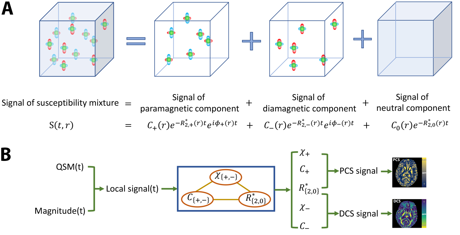
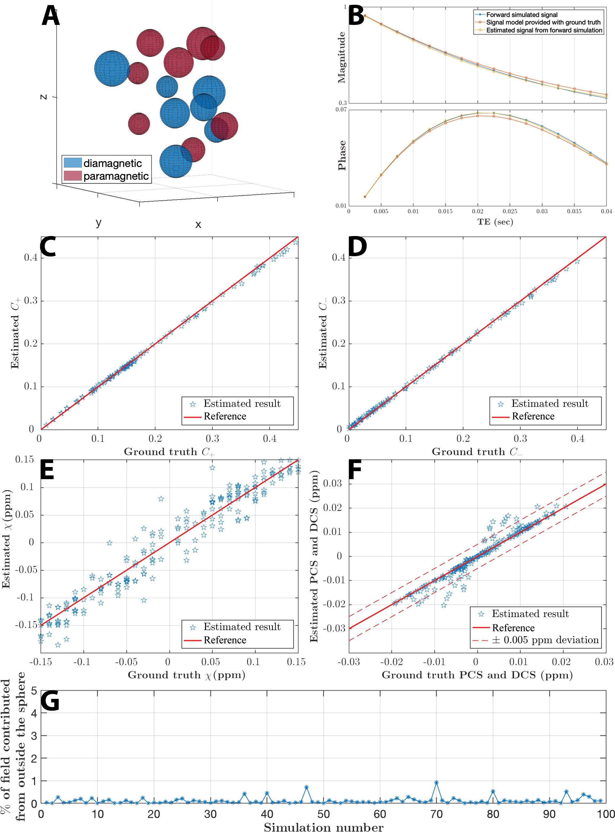
Figure 2. (A) Random assignments of susceptibility sources in a voxel space. (B) Complex signals from simulation, model with ground truth parameters and with estimated parameters. (C~E) Estimated parameters vs the ground truth. Red line indicates the case when estimation equals ground truth. (F) The composite paramagnetic and diamagnetic component susceptibilities (PCS and DCS) matches ground truths within 0.05 ppm deviation. (G) percentage of field perturbation from outside the sphere is negligible for each voxel simulation, which validates the voxel field approximation.