Introduction

Quantitative susceptibility mapping (QSM) algorithms assume that the resonance frequency shift is attributed only to the isotropic magnetic susceptibility.¹ However, additional sources such as susceptibility anisotropy² and chemical exchange (CE)³ have been demonstrated to exist. Susceptibility tensor imaging (STI) extended the QSM model to include susceptibility anisotropy, revealing fiber orientation information.⁴ Recently, a multi-directional approach for separating susceptibility and chemical exchange was developed, suggesting the potentials of developing a more complete model of frequency shift.⁵ In this study, a novel model that encompasses both Chemical Exchange and Susceptibility Tensor (ChEST) is proposed and an iterative algorithm that solves the inverse problem of the model is developed. Numerical simulation and in-vivo results are included.

Methods

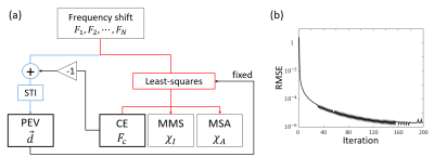
[ChEST model] The frequency shifts with N different B₀ directions in the subject frame of reference can be modeled as the sum of frequency shifts from chemical exchange and susceptibility tensor:^{4, 5}$$\triangledown{F_i}={FT}^{-1}\left\{\frac{1}{3}\overrightarrow{H}_i^TFT\left(\chi\right)\overrightarrow{H}_i-\overrightarrow{k}\cdot\overrightarrow{H}_i^T\frac{\overrightarrow{k}^TFT\left(\chi\right)\overrightarrow{H}_i}{\left|\overrightarrow{k}\right|^2}+FT\left(F_c\right)\right\},{\qquad}[Eq. 1]$$ where $$$FT$$$ and $$$FT^{-1}$$$ mean the Fourier transform and its inverse, $$$\overrightarrow{H}_i=\begin{bmatrix}H_{1i}&H_{2i}&H_{3i}\end{bmatrix}^T$$$ is the magnetic strength vector along each B₀ (i = 1,2,…, and N), $$$\triangledown{F_i}$$$ is the total frequency shift for the B₀ direction, $$$F_c$$$ is CE, and $$$\chi$$$ is the susceptibility tensor. CE is assumed to be orientation independent. This equation can be reformated as follows: $$\triangledown{F_i}={FT}^{-1}\begin{bmatrix}\frac{1}{3}H_{1i}^2-\overrightarrow{k}\cdot\overrightarrow{H}_i\frac{k_1H_{1i}}{\left|\overrightarrow{k}\right|^2}&\frac{2}{3}H_{1i}H_{2i}-\overrightarrow{k}\cdot\overrightarrow{H}_i\frac{k_1H_{2i}+k_2H_{1i}}{\left|\overrightarrow{k}\right|^2}&\cdots&\frac{1}{3}H_{3i}^2-\overrightarrow{k}\cdot\overrightarrow{H}_i\frac{k_3H_{3i}}{\left|\overrightarrow{k}\right|^2}\end{bmatrix}{FT}\begin{bmatrix}\chi_{11}\\\chi_{12}\\\chi_{13}\\\chi_{22}\\\chi_{23}\\\chi_{33}\\F_c\end{bmatrix}.{\qquad}[Eq. 2]$$ When multiple B₀ directional data are acquired, Equation 2 can be rewritten as follows:⁶ $$\begin{bmatrix}\triangledown{F_1}\\\triangledown{F_2}\\{\vdots}\\\triangledown{F_N}\end{bmatrix}={FT}^{-1}\begin{bmatrix}\frac{1}{3}H_{11}^2-\overrightarrow{k}\cdot\overrightarrow{H}_1\frac{k_1H_{11}}{\left|\overrightarrow{k}\right|^2}&\frac{2}{3}H_{11}H_{21}-\overrightarrow{k}\cdot\overrightarrow{H}_1\frac{k_1H_{21}+k_2H_{11}}{\left|\overrightarrow{k}\right|^2}&\cdots&\frac{1}{3}H_{31}^2-\overrightarrow{k}\cdot\overrightarrow{H}_1\frac{k_3H_{31}}{\left|\overrightarrow{k}\right|^2}\\\frac{1}{3}H_{12}^2-\overrightarrow{k}\cdot\overrightarrow{H}_2\frac{k_1H_{12}}{\left|\overrightarrow{k}\right|^2}&\frac{2}{3}H_{12}H_{22}-\overrightarrow{k}\cdot\overrightarrow{H}_2\frac{k_1H_{22}+k_2H_{12}}{\left|\overrightarrow{k}\right|^2}&\cdots&\frac{1}{3}H_{32}^2-\overrightarrow{k}\cdot\overrightarrow{H}_2\frac{k_2H_{32}}{\left|\overrightarrow{k}\right|^2}\\&&\vdots\\\frac{1}{3}H_{1N}^2-\overrightarrow{k}\cdot\overrightarrow{H}_N\frac{k_1H_{1N}}{\left|\overrightarrow{k}\right|^2}&\frac{2}{3}H_{1N}H_{2N}-\overrightarrow{k}\cdot\overrightarrow{H}_N\frac{k_1H_{2N}+k_2H_{1N}}{\left|\overrightarrow{k}\right|^2}&\cdots&\frac{1}{3}H_{3N}^2-\overrightarrow{k}\cdot\overrightarrow{H}_N\frac{k_3H_{3N}}{\left|\overrightarrow{k}\right|^2}\end{bmatrix}{FT}\begin{bmatrix}\chi_{11}\\\chi_{12}\\\chi_{13}\\\chi_{22}\\\chi_{23}\\\chi_{33}\\F_c\end{bmatrix}.{\qquad}[Eq. 3]$$ However, even with a large number of B₀ directions, the maximum rank of Equation 3 is still 6 because all components of the matrix can be represented as a linear combination of $$$H_{1i}^2$$$, $$$H_{2i}^2$$$, $$$H_{3i}^2$$$, $$$H_{1i}H_{2i}$$$, $$$H_{1i}H_{3i}$$$, $$$H_{2i}H_{3i}$$$ (i.e., $$$H_{1i}^2+H_{2i}^2+H_{3i}^2=1$$$). To overcome this rank deficiency, we posed an assumption that the anisotropy is cylindrically symmetric.⁷ Then, the susceptibility tensor ($$$\chi$$$) can be described as:$$\chi=(\chi_I-\frac{\chi_A}{3})I+\chi_A\overrightarrow{d}\overrightarrow{d}^T,{\qquad}[Eq. 4]$$ where $$$\chi_I$$$ is the mean magnetic susceptibility (MMS), $$$\chi_A$$$ is the magnetic susceptibility anisotropy (MSA), $$$I$$$ is an identity matrix, and $$$\overrightarrow{d}=\begin{bmatrix}d_1&d_2&d_3\end{bmatrix}^T$$$ is the principal eigenvector (PEV). Then, Equation 3 can be expressed as: $$\begin{bmatrix}\triangledown{F_1}\\\triangledown{F_2}\\{\vdots}\\\triangledown{F_N}\end{bmatrix}=A\begin{bmatrix}1\\0\\0\\1\\0\\1\end{bmatrix}\chi_I+A\begin{bmatrix}d_1^2-\frac{1}{3}\\{d_1d_2}\\{d_1d_3}\\d_2^2-\frac{1}{3}\\{d_2d_3}\\d_3^2-\frac{1}{3}\end{bmatrix}\chi_A+\begin{bmatrix}1\\1\\{\vdots}\\1\end{bmatrix}F_c,{\qquad}[Eq. 5]$$ where $$$A={FT}^{-1}\begin{bmatrix}\frac{1}{3}H_{11}^2-\overrightarrow{k}\cdot\overrightarrow{H}_1\frac{k_1H_{11}}{\left|\overrightarrow{k}\right|^2}&\frac{2}{3}H_{11}H_{21}-\overrightarrow{k}\cdot\overrightarrow{H}_1\frac{k_1H_{21}+k_2H_{11}}{\left|\overrightarrow{k}\right|^2}&\cdots&\frac{1}{3}H_{31}^2-\overrightarrow{k}\cdot\overrightarrow{H}_1\frac{k_3H_{31}}{\left|\overrightarrow{k}\right|^2}\\\frac{1}{3}H_{12}^2-\overrightarrow{k}\cdot\overrightarrow{H}_2\frac{k_1H_{12}}{\left|\overrightarrow{k}\right|^2}&\frac{2}{3}H_{12}H_{22}-\overrightarrow{k}\cdot\overrightarrow{H}_2\frac{k_1H_{22}+k_2H_{12}}{\left|\overrightarrow{k}\right|^2}&\cdots&\frac{1}{3}H_{32}^2-\overrightarrow{k}\cdot\overrightarrow{H}_2\frac{k_2H_{32}}{\left|\overrightarrow{k}\right|^2}\\&&\vdots\\\frac{1}{3}H_{1N}^2-\overrightarrow{k}\cdot\overrightarrow{H}_N\frac{k_1H_{1N}}{\left|\overrightarrow{k}\right|^2}&\frac{2}{3}H_{1N}H_{2N}-\overrightarrow{k}\cdot\overrightarrow{H}_N\frac{k_1H_{2N}+k_2H_{1N}}{\left|\overrightarrow{k}\right|^2}&\cdots&\frac{1}{3}H_{3N}^2-\overrightarrow{k}\cdot\overrightarrow{H}_N\frac{k_3H_{3N}}{\left|\overrightarrow{k}\right|^2}\end{bmatrix}FT$$$. To resolve the multiplication between $$$\overrightarrow{d}$$$ and $$$\chi_A$$$ in the equation, an iterative method is developed to estimate $$$\chi_I$$$, $$$\chi_A$$$, $$$\overrightarrow{d}$$$, and $$$F_c$$$ . The iteration consists of two steps. In the first step, STI is performed with fixed $$$F_c$$$, and then the principal eigenvector $$$\overrightarrow{d}$$$ is calculated by eigenvalue decomposition. In the second step, with $$$\overrightarrow{d}$$$ fixed, $$$\chi_I$$$, $$$\chi_A$$$, and $$$F_c$$$ are fitted with Equation 5 using the least-squares method. These two steps are iterated until the difference between measured frequency shift and predicted frequency shift are less than a threshold, producing MMS, MSA, PEV, and CE (Fig. 1a).
[Simulation] A brain-shaped phantom is designed with the cylindrically symmetric susceptibility tensor and chemical exchange. The chemical exchange is assumed to have a lower contrast range than that of MMS referenced from a recent study⁵ (e.g. iron oxide: CE = -39 ppb and susceptibility = 300 ppb). Then, twelve directional datasets are generated ( $$$\theta$$$ = [0°, 17.2°, 23.5°, 15.5°, 24.2°, 7.9°, 12.9°, 15.1°, 13.9°, 20.7°, 20.8°, 25.4°] and $$$\phi$$$ = [0°, -14°, -32.5°, -155°, -153.2°, 85.1°, 12.9°, -179.7°, -96.4°, -88.4°, -76.2°, -111.4°]). The ChEST is applied to reconstruct the MMS, MSA, PEV, and CE maps. Simulation is conducted with and without Gaussian noise (SNR = 100). A conjugate gradient algorithm (tolerance: 10^-3) is used for least-squares estimation with regularization to constrain MSA in white matter similar to MMSR-STI⁸ ( $$$\alpha=10$$$). It takes 200 iterations to converge (Fig. 1b). For comparison, MMSR-STI⁸ and STI⁴ reconstructions are also performed.
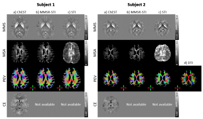
[In-vivo application] To demonstrate the feasiblity of applying ChEST to in-vivo data, two existing datasets are utilized (Subject 1: 12 directional QSM challenge 2016 data;⁹ Subject 2: 12 directions, 3D GRE, FOV = 216×216×216 mm³, resolution = 1.5×1.5×1.5 mm³, TR/TE = 40/25 ms, FA = 15° , TA = 11:03 per acquisition.⁸)

Results

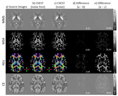
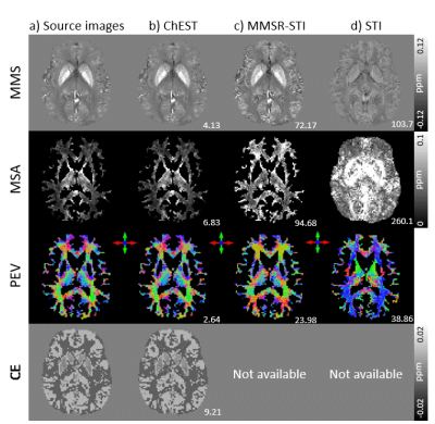
As demonstrated in Figure 2, the proposed ChEST method successfully reconstructs MMS, MSA, PEV, and CE maps in the noise-free condition. Even with additive Gaussian noise, ChEST produces all maps with small errors. Figure 3 illustrates the comparison results for the ChEST and conventional algorithms. When compared to the conventional STI algorithms that exclude the chemical exchange in their models, the proposed method generates the maps with lower NRMSE values. In Figure 4, the in-vivo results are displayed. The CE map shows a much smaller contrast range compared to those of MMS and MSA, confirming our previous assumption in QSM that the contribution of CE is much smaller than that of susceptibility. The other susceptibility-related maps are consistent with MMSR-STI.

Conclusion and Discussion

In this study, we introduced an integrated model for frequency shift, proposing ChEST, a novel method that estimates both chemical exchange and susceptibility tensor. Compared to the previous approaches, our method successfully reconstructs MMS, MSA, PEV, and CE maps. In the in-vivo results, the CE map showed a smaller contrast range than the MMS and MSA maps, agreeing with our recent measurements.⁵

Acknowledgements

This work was supported by the National Research Foundation of Korea (NRF) grant funded by the Korea government(MSIT) (No. NRF-2018R1A2B3008445, NRF-2017M3C7A1047864).