0785
DeepControl: AI-powered slice flip-angle homogenization by 2DRF pulses1Center of Functionally Integrative Neuroscience, Aarhus University, Aarhus, Denmark, 2Physikalisch-Technische Bundesanstalt (PTB), Braunschweig and Berlin, Germany, 3Harvard Medical School, Boston, MA, United States, 4Martinos Center for Biomedical Imaging, Massachusetts General Hospital, Charlestown, MA, United States, 5Center for Magnetic Resonance Research, University of Minnesota, Minneapolis, MN, United States
Synopsis
We test the DeepControl convolutional neural network for brain slice 2DRF 30o excitations (single-channel) at 7 T with a uniform FA profile. While the DeepControl framework was originally designed for localized 2D spatial-selective excitations, we demonstrate robustness towards FA homogenization at 7 T. Our numerical study, a comparison to gradient-ascent-pulse-engineering optimal control pulses, shows good pulse performance and (near-)conformity to the optimal control training library, including the RF pulse constraints. The DeepControl pulse prediction time takes only ~9 ms, which is more than 1000 times faster than the optimal control.
Introduction
At $$$7\,\mathrm{T}$$$, non-uniform B1+ fields generate regions with lower flip angles (FAs), which negatively impact signal and contrast. Spokes1, kT-points2, and SPINS3 pulses achieve homogeneous excitation despite non-uniform B1+ fields, with further benefit using pTx4–6 or B0-shim arrays7, e.g. with fast-switching, arbitrary-waveform, INSTANT pulses8,9. Optimal control (OC) 2DRF (or 3DRF) pulses based on spiral kx-ky trajectories have been proposed by our group10,11 and others12,13, which further enable arbitrary selection patterns. However, patient-tailored pulses need fast computation to be applicable in vivo14. We have recently shown, in vivo at $$$7\,\mathrm{T}$$$, that a convolutional neural network "DeepControl" in only $$$9\,\mathrm{ms}$$$ can predict OC-like 2DRF-pulses able to excite arbitrary shapes15. Here, we demonstrate the ability of the method to generate uniform FA excitations in the brain at $$$7\,\mathrm{T}$$$.Methods
2DRF: The inward, 16-turn spiral trajectory (duration:$$$\,7\,\mathrm{ms}$$$, dwell:$$$\,\Delta t=10\,\mu\mathrm{s,}\,$$$max$$$\,40\,\mathrm{mT/m},\,180\,\mathrm{T/m/s,\,}$$$field of excitation$$$\,25\,\mathrm{cm}$$$) was fixed in all the pulse optimizations in this work.Training Library: Our library was composed of 500k “examples” of B1+, B0 and target excitation profiles including their OC-computed “reference” pulses10,11. Each of three input maps, are fixed to a $$$64\times64$$$ matrix ($$$25\times25\,\mathrm{cm}^2$$$). The first is a $$$30^\circ\,$$$target-FA pattern (a polygon from ten randomly placed points was closed morphologically to one arbitrary shape with no holes). The second is the B0 map (random photographs from ImageNet, cropped, shifted (so the average pixel value is 0), and then scaled to a maximum value being a random number in the range $$$\left[50\,\mathrm{Hz};\,600\,\mathrm{Hz}\right]$$$. The third input is the (magnitude) B1+ map (random photographs from ImageNet, cropped and normalized as a sensitivity map with range $$$[0;\,1]\,\sim\,[0;\,196\,\mathrm{nT/V}]$$$).
Optimal control: We used the gradient-ascent-pulse-engineering16 OC framework "blOCh”10,11 for computing RF library$$$\,+\,$$$experiment pulses ($$$50\,$$$iterations, tolerances$$$\,1\cdot10^{-6}$$$). The real/imaginary amplitude of the RF pulse were constrained to$$$\,1\,\mathrm{kHz}\sim\,120\,\mathrm{V}$$$.
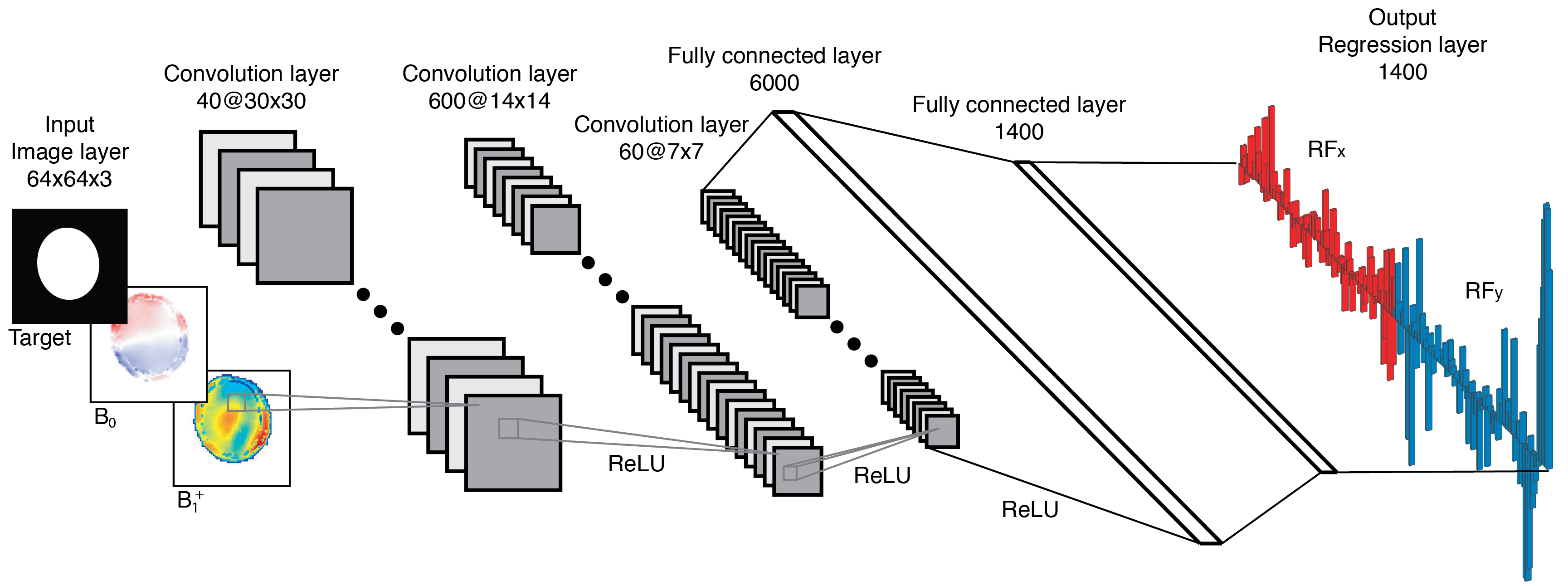
DeepControl: The deep convolutional neural network in Fig.$$$\,1$$$ was trained with the stochastic-gradient-descent-with-momentum algorithm (MATLAB), with validation every$$$\,1000\,$$$iterations. Training was stopped manually upon convergence after$$$\,229\,\mathrm{epochs}\,\sim\,36\,\mathrm{hours}$$$. The mini-batch size and initial learn rate were$$$\,1024\,$$$and$$$\,0.006$$$, respectively. Library input/output pairs were shuffled.
Experiments: MRI was performed on a $$$7\,\mathrm{T}$$$ Magnetom (Siemens Healthineers, Erlangen, Germany), with 8 channels$$$(1\,\mathrm{kW/ch.})\,$$$driven in circularly-polarized (CP) mode on a healthy female volunteer (supine) under approved IRB.
The actual-flip-angle17 B1+ mapping parameters (obtained for the CP-mode of the pTx-array) were:
$$$\mathrm{FA}_\mathrm{nominal}=90^\circ$$$,$$$\,\mathrm{TE/\,TR}_1/\,\mathrm{TR}_2=2.64/\,20/\,120\,\mathrm{ms}$$$,$$$\,\mathrm{FOV}\,:\,\mathrm{RO}\times\mathrm{PE}\times\mathrm{PE}_2=250\times250\times192\,\mathrm{mm}^3,\,$$$matrix:$$$\,\mathrm{RO}\times\mathrm{PE}\times\mathrm{PE}_2=64\times64\times48,\,10\,\mathrm{min}\,5\,\mathrm{s}$$$.
The 3D GRE B0 mapping parameters were:
$$$\mathrm{FA}_\mathrm{nominal}=30^\circ$$$,$$$\,\mathrm{TE}_1/\,\mathrm{TE}_2/\,\mathrm{TR}=3.06/\,4.08/\,500\,\mathrm{ms},\,$$$FOV:$$$\,\mathrm{RO}\times\mathrm{PE}\times\mathrm{PE}_2=250\times250\times192\,\mathrm{mm}^3,\,$$$matrix:$$$\,\mathrm{RO}\times\mathrm{PE}\times\mathrm{PE}_2=64\times64\times48$$$,$$$\,1\,\mathrm{min}\,7\,\mathrm{s}$$$.
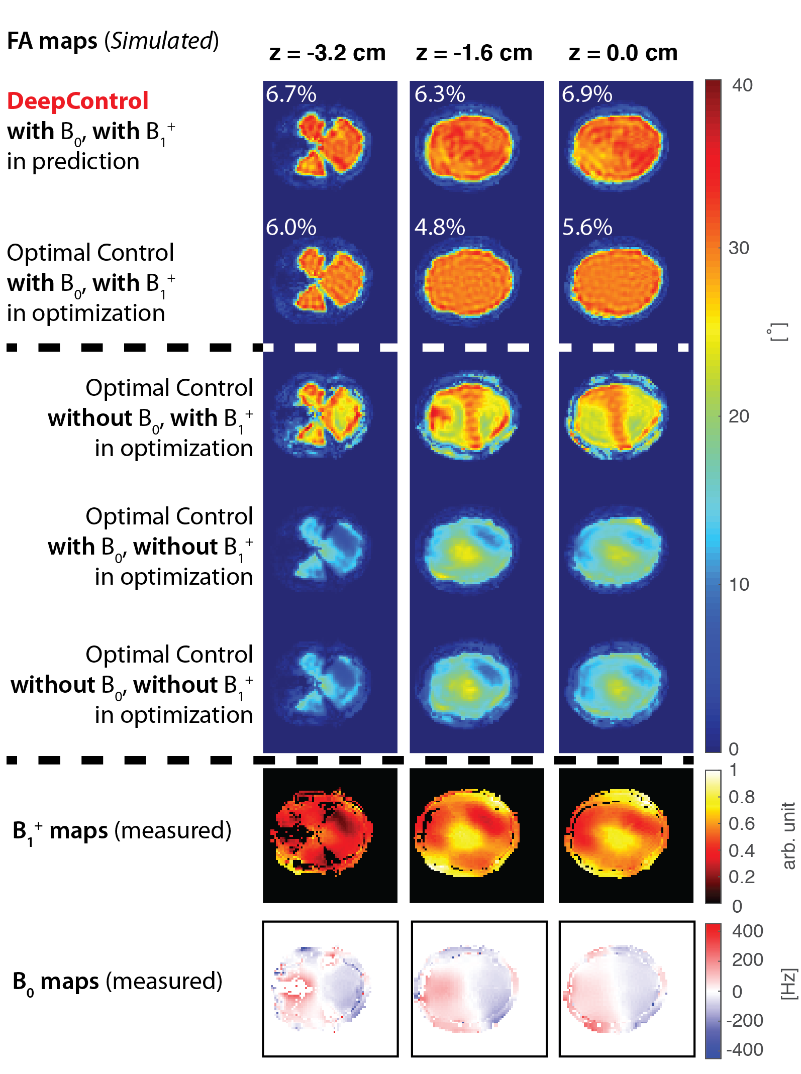
Simulations: For slice positions$$$\,z=-3.2,\,-1.6,\,$$$and$$$\,0\,\mathrm{cm}$$$ (from iso-center) extracted brain masks were used as FA targets. We optimized four sets of OC pulses: One with B1+ and B0 maps included, one with both maps replaced with ideal conditions$$$\,\Delta B_0(\mathbf{r}) = 0$$$,$$$\,B_1^+(\mathbf{r}) = 1,\,\forall\,\mathbf{r}$$$, and two, where either the B0 or the B1+ map was replaced with ideal conditions, vice versa.
Results
The OC computations in this study took around 20 seconds each on a laptop. The DeepControl prediction times were around $$$9\,\mathrm{ms}\,$$$i.e. more than$$$\,1000\times\,$$$faster.Fig.$$$\,2$$$ shows the FA maps for pulses generated for the three brain mask targets ($$$z=-3.2,\,-1.6\,$$$and$$$\,0\,\mathrm{cm}$$$) and their corresponding B1+/B0 maps. The DeepControl (first row) compensates, like OC (second row), the B1+ inhomogeneities, with just a small increase in normalized root-mean-square-error,$$$\,1-2\%$$$, approximately (printed numbers).
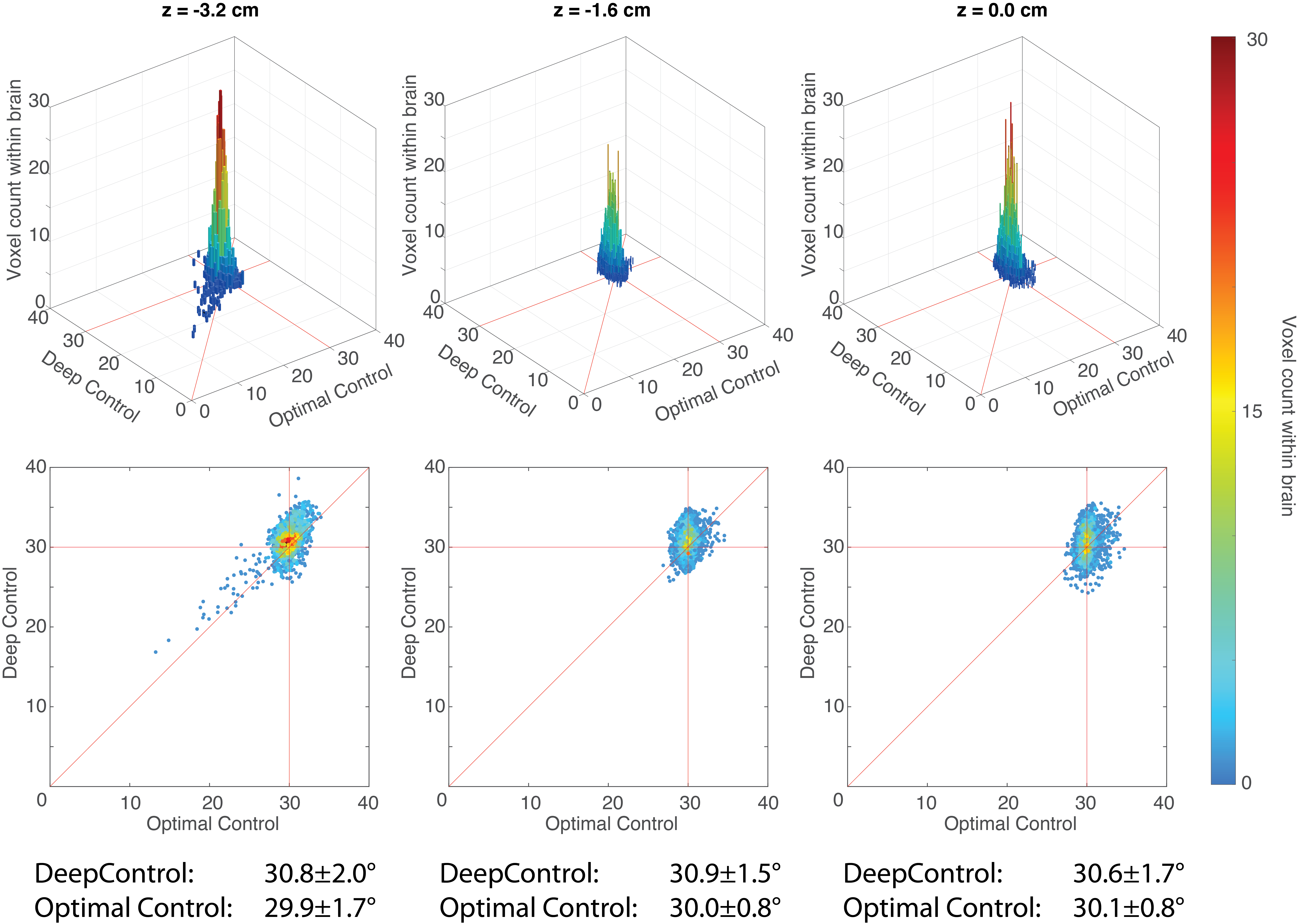
Fig.$$$\,3\,$$$shows the 3D/2D histograms of DeepControl vs. OC. Centered close to $$$\mathrm{FA}_{\mathrm{nominal}}=30^\circ$$$, the mean and standard deviation of the FA values for OC and DeepControl are very similar.
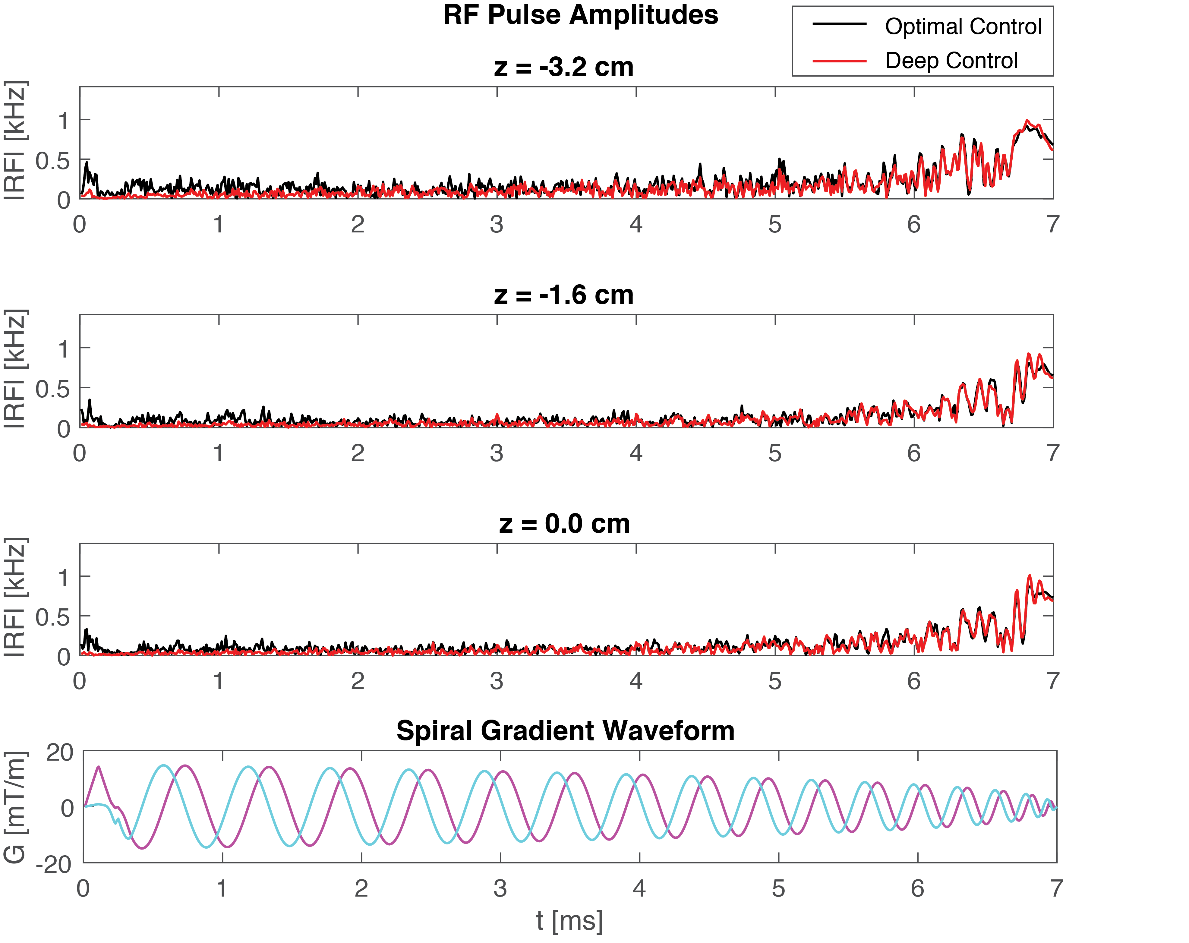
Fig.$$$\,4\,$$$shows DeepControl pulse waveforms (red) overlayed with the corresponding OC waveforms (black). The DeepControl pulse (imaginary part) for $$$z=0\,\mathrm{cm}$$$ overshoots the $$$1\,\mathrm{kHz}$$$ limit by only $$$\sim0.5\%$$$, showing that the DeepControl was able to learn not only the OC design, but also the constraints.
Discussion
The DeepControl convolutional neural network was designed for custom/local shape excitation, but herein we demonstrate its usefulness for flip-angle homogenization in the brain at $$$7\,\mathrm{T}$$$.Row three to five in Fig.$$$\,2$$$ show that missing field information in OC optimizations does not yield good results. In practice, accurate B1+ and B0 maps should be presented to the network. In Ref.14, we presented a neural network, which did not include field maps in the input (only the target pattern). Applied here, the missing field information would impart the same kind of distortions (data not shown).
Only small increases in FA variations were observed in the plane by using the proposed version of DeepControl. In future work, we aim at verifying these results in experiments.
We will also study the impact of extension of the training library on the quality of the excitations, especially by adding "brain-like" target cases, and more realistic B1+ maps to the training set18.
There is presently no explicit handle on RF power in DeepControl, but clearly it seems sufficient to add the constraints in the training set. For the (20%) test subset of the DeepControl library (500k cases in total), we observed overshoot (median 7.3%) in only 2% of the cases15. The small overshoot is easily dealt with, e.g., by lowering the peak voltage constraint in the library or by using VERSE19.
Conclusion
A rapid ($$$9\,\mathrm{ms}$$$ prediction time) single-channel 2DRF pulse design framework, DeepControl, was demonstrated with numerical simulations for brain shape excitations and FA homogenization at $$$7\,\mathrm{T}$$$.Acknowledgements
MSV and TEL wish to thank Villum Fonden, Eva og Henry Frænkels Mindefond, Harboefonden and Kong Chr. den Tiendes Fond.References
1. Saekho, S., Yip, C., Noll, D. C., Boada, F. E. & Stenger, V. A. Fast-kz three-dimensional tailored radiofrequency pulse for reducedB1 inhomogeneity. Magnetic Resonance in Medicine 55, 719–724 (2006).
2. Cloos, M. A. et al. kT-points: Short three-dimensional tailored RF pulses for flip-angle homogenization over an extended volume. Magnetic Resonance in Medicine 67, 72–80 (2012).
3. Malik, S. J., Keihaninejad, S., Hammers, A. & Hajnal, J. V. Tailored excitation in 3D with spiral nonselective (SPINS) RF pulses. Magnetic Resonance in Medicine 67, 1303–1315 (2012).
4. Katscher, U., Börnert, P., Leussler, C. & van den Brink, J. S. Transmit SENSE. Magnetic Resonance in Medicine 49, 144–150 (2003).
5. Zhu, Y. Parallel excitation with an array of transmit coils. Magnetic Resonance in Medicine 51, 775–784 (2004).
6. Padormo, F., Beqiri, A., Hajnal, J. V. & Malik, S. J. Parallel transmission for ultrahigh-field imaging: Parallel Transmission for Ultrahigh-Field Imaging. NMR in Biomedicine 29, 1145–1161 (2016).
7. Umesh Rudrapatna, S., Juchem, C., Nixon, T. W. & de Graaf, R. A. Dynamic multi-coil tailored excitation for transmit B1correction at 7 Tesla: Dynamic Multi-coil Tailored Excitation. Magnetic Resonance in Medicine 76, 83–93 (2016).
8. Stockmann, J. P. & Wald, L. L. In vivo B 0 field shimming methods for MRI at 7 T. NeuroImage 168, 71–87 (2018).
9. Vinding, M. S., Lund, T. E., Stockmann, J. P. & Guerin, B. INSTANT (INtegrated Shimming and Tip-Angle NormalizaTion): 3D flip-angle mitigation using joint optimization of RF and shim array currents. in Proc. Intl. Soc. Magn. Reson. Med. 28 0612 (2020).
10. Vinding, M. S., Guérin, B., Vosegaard, T. & Nielsen, N. Chr. Local SAR, global SAR, and power-constrained large-flip-angle pulses with optimal control and virtual observation points. Magnetic Resonance in Medicine 77, 374–384 (2017).
11. Vinding, M. S., Maximov, I. I., Tošner, Z. & Nielsen, N. Chr. Fast numerical design of spatial-selective rf pulses in MRI using Krotov and quasi-Newton based optimal control methods. The Journal of Chemical Physics 137, 054203 (2012).
12. Grissom, W. et al. Spatial domain method for the design of RF pulses in multicoil parallel excitation. Magnetic Resonance in Medicine 56, 620–629 (2006).
13. Xu, D., King, K. F., Zhu, Y., McKinnon, G. C. & Liang, Z.-P. Designing multichannel, multidimensional, arbitrary flip angle RF pulses using an optimal control approach. Magnetic Resonance in Medicine 59, 547–560 (2008).
14. Vinding, M. S., Skyum, B., Sangill, R. & Lund, T. E. Ultrafast (milliseconds), multidimensional RF pulse design with deep learning. Magnetic Resonance in Medicine 82, 586–599 (2019).
15. Vinding, M. S., Aigner, C. S., Schmitter, S. & Lund, T. E. DeepControl: 2DRF pulses facilitating B1+ inhomogeneity and B0 off-resonance compensation in vivo at 7T. Magnetic Resonance in Medicine, Accepted (2020).
16. Khaneja, N., Reiss, T., Kehlet, C., Schulte-Herbrüggen, T. & Glaser, S. J. Optimal control of coupled spin dynamics: design of NMR pulse sequences by gradient ascent algorithms. Journal of Magnetic Resonance 172, 296–305 (2005).
17. Yarnykh, V. L. Actual flip-angle imaging in the pulsed steady state: A method for rapid three-dimensional mapping of the transmitted radiofrequency field. Magnetic Resonance in Medicine 57, 192–200 (2007).
18. Tomi‐Tricot, R. et al. SmartPulse, a machine learning approach for calibration‐free dynamic RF shimming: Preliminary study in a clinical environment. Magnetic Resonance in Medicine 82, 2016–2031 (2019).
19. Conolly, S., Nishimura, D., Macovski, A. & Glover, G. Variable-rate selective excitation. Journal of Magnetic Resonance (1969) 78, 440–458 (1988).
Figures