0783
Inner Volume Excitation via Joint Design of Time-varying Nonlinear Shim-array Fields and RF Pulse1Department of Electrical Engineering and Computer Science, Massachusetts Institute of Technology, Cambridge, MA, United States, 2Athinoula A. Martinos Center for Biomedical Imaging, Charlestown, MA, United States, 3Harvard-MIT Health Sciences and Technology, Massachusetts Institute of Technology, Cambridge, MA, United States, 4Institute for Medical Engineering and Science, Massachusetts Institute of Technology, Cambridge, MA, United States
Synopsis
Inner volume excitation is a promising technique to save scanning time or improve spatial resolution. Shim arrays provide nonlinear fields that extend the possibility of RF excitation of complicated spatial patterns. Yet previous work only employed static non-linear B field and predefined RF pulse which limits the performance. Validated on a fairly difficult tailored 3d volume pattern, jointly designed time-varying nonlinear B field and RF pulse within the auto-differentiable Bloch simulator framework shows substantial improvements. The accuracy improves 62% in terms of L2 norm with incorporated constraints on available RF pulse power.
Introduction
Magnetic resonance imaging of the fetus is challenged by fetal and maternal motion, and is thus typically limited to single-shot imaging techniques such as HASTE1 or SS-FSE. Slice-selective excitation2 for imaging of the fetal brain would benefit from methods for localized, inner-volume excitation patterns by reducing the encoding burden, and improve contrast or spatial resolution. Nonlinear fields generated by shim arrays3 have been demonstrated for spatially-selective excitation in the adult brain only with static shim-array fields with predefined RF pulse. Compared with previous work, we present numerical simulations of localized, inner-volume excitation of a spherical pattern designed by a joint optimization of a set of time-varying, spatially-nonlinear shim array fields and a time-varying RF pulse. This problem is challenging, as inverting the Bloch simulation poses a non-linear, non-convex objective function. Here, we exploit recent work5 with an auto-differentiable Bloch simulator to estimate the implicit Jabobian. The resulting excitation, due to the shim-array fields and RF pulse, but in the absence of linear gradient fields, achieves desired excitation pattern and improves the performance up to 62%.Method
The AC/DC shim array is designed to provide B0 shimming while preserving the array’s reception sensitivity. Each coil will generate a B0 field pattern which is non-linear in space and the field strength in each space grid is only related to the current. Thus, it could be further utilized for inner volume excitation by modifying the spatial B0 distribution inside and outside the desired region by the formulation proposed in previous work4. However, the performance is below the expectation due to maximum modulus principle which explains the formulation in work4 fails to obtain the desirable excitation pattern as some parts of the actually excited region tend to touch the boundary of FOV.To mitigate this problem, one way is to fully exploit the advantages of readout direction and aliasing rules by modifying the desired excitation pattern with don’t care region. In this work, we present the ability of time-varying nonlinear fields by employing the auto-differentiation directly to the time-discrete Bloch simulator as proposed in recent work5. Compared with their work, we incorporate the non-linear B field by The formulation is shown as below,
$$\underset{I \in \mathbb{R}^{n_{T} \times 32}, b \in \mathbb{C}^{n_{T} }}{\arg \min } \quad \mathcal{L} =f\left(W * M_{xy}(I, b), W * M_{D}\right)+ \mathcal{R}(b)$$
where $$$M_D$$$ is the desired excitation pattern, $$$M_{xy}$$$ is the actual excitation profile generated by the RF and time-varying nonlinear B field using time-discrete Bloch simulator. $$$W$$$ is the loss weight of different inner and outer volumes. $$$\mathcal{R}(b)$$$ is the regularizer to limit the RF power where we used Tikhonov regularizer in this work. $$$I$$$ is the current, $$$b$$$ is the Rf pulse, $$$n^T$$$ is the number of time point and $$$32$$$ is the number of shim coil.
As the formulation is non-linear and non-convex, the initialization is of vital importance to avoid being trapped in suboptimal solution. Besides, to make the formulation more robust to initialization, a good choice of loss weight is the inverse proportion of the number of volumes inside and outside the desired excitation pattern
Results and Discussions
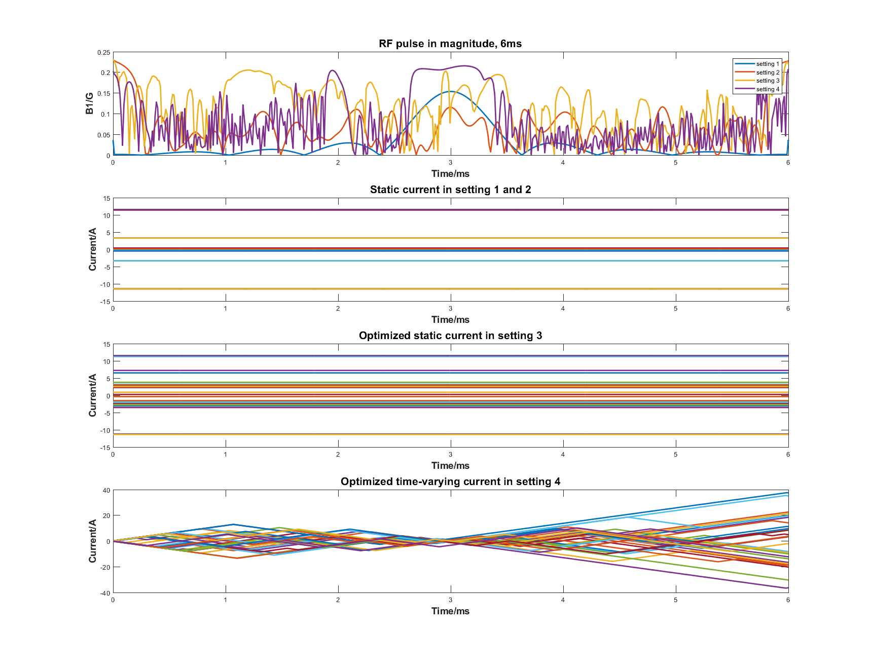
Shown in figure 1, in this work, we conduct the validation experiments on a 32*32*32 voxel grid with FOV of 24*24*24 cm3. To fully present the ability of the proposed method, the desired excitation pattern is a 3D ball (radius = 3.57cm) which is set to 1/3 of the FOV. We use 32 shim coils. The maximum current limitation is 50A per coil and the slew rate of the current is 35000A/s. bmax = 0.25G.We perform the experiments mainly on four different settings. If not clarified, the initialization is the optimized result of setting 1.
1. Static non-linear B field with sinc shape RF pulse optimized by the method described in work4.
2. Same static non-linear B field as setting 1 with only optimized RF pulse.
3. Joint optimized static non-linear B field and RF pulse.
4. Joint optimized time-varying nonlinear B field and rf pulse. The initialized pattern is uniformly $$$|M_{xy}| = 0.5$$$ within the whole volume.
The results could be seen from figure 2. The proposed method achieves the least error where the excited pattern is the most desirable one. Also seen from figure 3, compared with the static non-linear B field, the proposed method acquires more current which uses the non-linear field more efficiently.
We also conduct experiments on setting 3 and 4 using different initializations. There are two initializations, one is the result of setting 1, another one is uniformly distributed $$$|M_{xy}| = 0.5$$$. Seen from figure 4, the excitation result is more robust than that of setting 3 with different RF and current levels.
Conclusions
Shim arrays provide non-linear B fields to modify the spatial resonance distribution and offer new degrees of freedom for RF excitation designs. In this abstract we proposed a novel method by adopting the auto-differentiable Bloch simulator to jointly design the time-varying nonlinear B field and corresponding RF pulses and thus extended prior work that applied static shim-array fields and a predefined sinc shape RF pulse. The results show substantial improvements with time-varying fields and suggest further applications for more complex excitation patterns.Acknowledgements
This work was supported in part by research grants NIH R01 EB017337, U01 HD087211, R01HD100009.References
1. Patel, Mahesh R., et al. "Half-fourier acquisition single-shot turbo spin-echo (HASTE) MR: comparison with fast spin-echo MR in diseases of the brain." American journal of neuroradiology 18.9 (1997): 1635-1640.
2. Feinberg, David A., et al. "Inner volume MR imaging: technical concepts and their application." Radiology 156.3 (1985): 743-747.
3. Stockmann, Jason P., et al. "A 32‐channel combined RF and B0 shim array for 3T brain imaging." Magnetic resonance in medicine 75.1 (2016): 441-451.
4. Stockmann, J., et al. "Spatially-selective excitation using a tailored nonlinear ΔB0 pattern generated by an integrated multi-coil ΔB0/Rx array." Int. Soc. Magn. Reson. Med. Vol. 170. 2018.
5. Luo, Tianrui, et al. "Joint Design of RF and gradient waveforms via auto-differentiation for 3D tailored excitation in MRI." arXiv preprint arXiv:2008.10594 (2020).
Figures
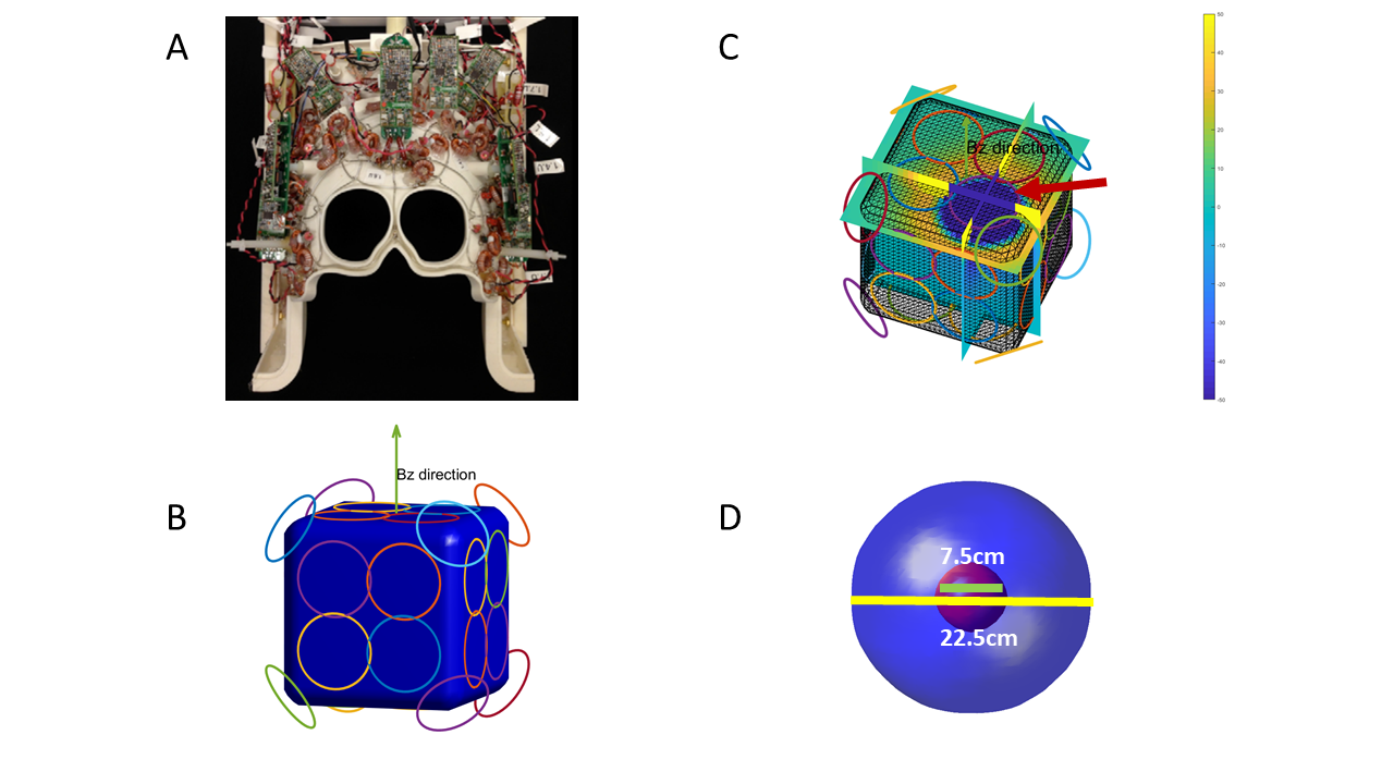
A. The head shim array using 32 coils.
B. 32 coils used in this simulation. 24 coils are uniformly distributed on the 6 surfaces and 8 coils are distributed on the vertexes.
C. The Bz field pattern generated by the coil under the right arrow under 1A.
D. The desired excited pattern (red ball) and suppressed background (blue ball). The diameter of the red ball is 1/3 of that of the background ball.