Introduction

QSM is a valuable phase-based post-processing technique, which quantifies the magnetic susceptibility distribution of biological tissues. QSM scans are generally acquired with GRE¹ or SWI² sequences, which are relatively slow. Compressed sensing (CS) undersampling and reconstruction have been used to accelerate magnitude-based MRI scans^3-6. However, these methods are not applicable to the phase. In this study, we propose a complex attention network, named CANet, via incorporating complex convolutional layers and complex attention modules, to recover both MR magnitude and quantitative phase images, thus enabling the acceleration of QSM acquisitions. Magnitude, phase, and QSM results from CANet will be compared with a recent compressed sensing phase cycling (CSPC)⁷ reconstruction algorithm.

Methods

CANet
The overall QSM accelerating framework and the architecture of the proposed CANet are shown in Figure 1. The CANet is built on the residual network backbone by adding complex convolutional layers and complex attention modules. As illustrated in Figure 2(a), the complex convolution can be formulated as:
Y=X\divideontimes W$ where $ \left\{\begin{matrix}Y=\ Y_R+\ i\ Y_I\ \\Y_R=\ X_R\ast W_R+X_I\ast W_I\\Y_I=\ X_R\ast W_I+X_I\ast W_R\\\end{matrix}\right.
where $\divideontimes$ represents the complex-valued convolution and * represents the conventional real-valued convolution in traditional CNNs; X is the input, W is the complex convolutional kernels, and Y is the output.
Figure 2(b) and (c) depict the data flow of the proposed complex attention framework, consisting of two sequentially stacked sub-modules: i) channel attention module and ii) spatial attention module, which is formulated as:
\begin{matrix}Atten\left(X\right)=M_S\left(X_C\right)\bigotimes X_C\\{X_C=M}_C(X)\bigotimes X\\\end{matrix}
where $\bigotimes$ denote the element-wise complex multiplication, M_C and M_S are the 1D channel and 2D spatial attention maps, respectively. M_C is computed as:
\begin{matrix}M_C(X)=\sigma\left(MLP\left(MaxPool\left(X\right)\right)+MLP\left(AvgPool\left(X\right)\right)\right)\\MLP\left(a\right)=W_2\divideontimes(W_1\divideontimes a)\\\end{matrix}
where $\sigma$ is the sigmoid activation function; W₁ and W₂ are the kernels of the MLP; MaxPool and AvgPool are the global MaxPooling and AvgPooling operations. Ms can then be expressed as:
\begin{matrix}M_S\left(X\right)=\sigma\left(W_S\divideontimes D(X)\right)\\D\left(X\right)=\ concat(MaxPool\left(X,\ \prime C\prime\right),AvgPool\left(X,\prime C\prime\right))\\\end{matrix}
where W_s is the complex convolutional kernel; Concat, MaxPool(, 'C'), and AvgPool(, 'C') denote the concatenation, MaxPooling, and AvgPooling operations along the channel dimension.
The proposed CANet comprises 11 complex convolutional layers, 5 complex attention modules, and 1 final convolutional output layers. To train the proposed CANet, a total of 50,400 brain complex-valued images (size: 256×128) were generated from 30 GRE scans, which were acquired with 1 mm isotropic voxel size, 256×256×128 mm³ FOV at 3T. All network parameters were initialized with normally distributed random numbers of zero mean and 0.01 standard deviation. Adaptive moment estimation was used to optimize the network. It took around 40 hours (i.e.,100 epochs) to complete the network training on two Tesla V100 GPUs using Pytorch 1.0, with the mini-batch size of 32 and MSE as the loss function.
Validation with Human Brain Datasets
Qualitative and quantitative comparisons are performed between the proposed CANet and CSPC algorithms on the magnitude, phase, and QSM images acquired from 4 healthy subjects (1 mm isotropic at 3T, FOV: 256×256×132 mm³), 1 intracranial hemorrhage (ICH) patient (1 mm isotropic at 3T, FOV: 226×226×120 mm³), and 1 multiple sclerosis (MS) patient (1 mm isotropic at 3T, FOV: 256×256×132 mm³). All k-space data were retrospectively undersampled with a factor of 4× with a 2D variable density undersampling mask⁸.

Results

Figure 3 compared zero-filling, CSPC and the proposed CANet results on a healthy human brain data. The magnitude, phase, local field maps (by RESHARP⁹), QSM (by xQSM¹⁰) and their corresponding error maps are reported from top to bottom. The CANet led to the most accurate reconstructions with the smallest error maps and the best PSNR and SSIM (e.g., 43.83/0.98 for QSM reconstructions). The bar graph in Figure 3 (c) compared the QSM measurements of one deep white matter and six deep grey matter regions from different CS reconstruction methods using four human subjects, which confirmed CANet leading to the most accurate quantitative results.
The CANet and CSPC were also applied to an ICH patient in Figure 4. As shown in Figure 4(a), the CSPC resulted in an over-smoothed reconstruction. In addition to the numerical metrics (i.e., PSNR and SSIM), the scatter plots and the linear regression results reported in Figure 4(b) and (c) demonstrated that the CANet (R²: 0.65, SSE: 1.89) led to the most accurate brain hemorrhage susceptibility measurements against the fully-sampled ground truth, as compared with CSPC (R²: 0.46, SSE: 2.28).
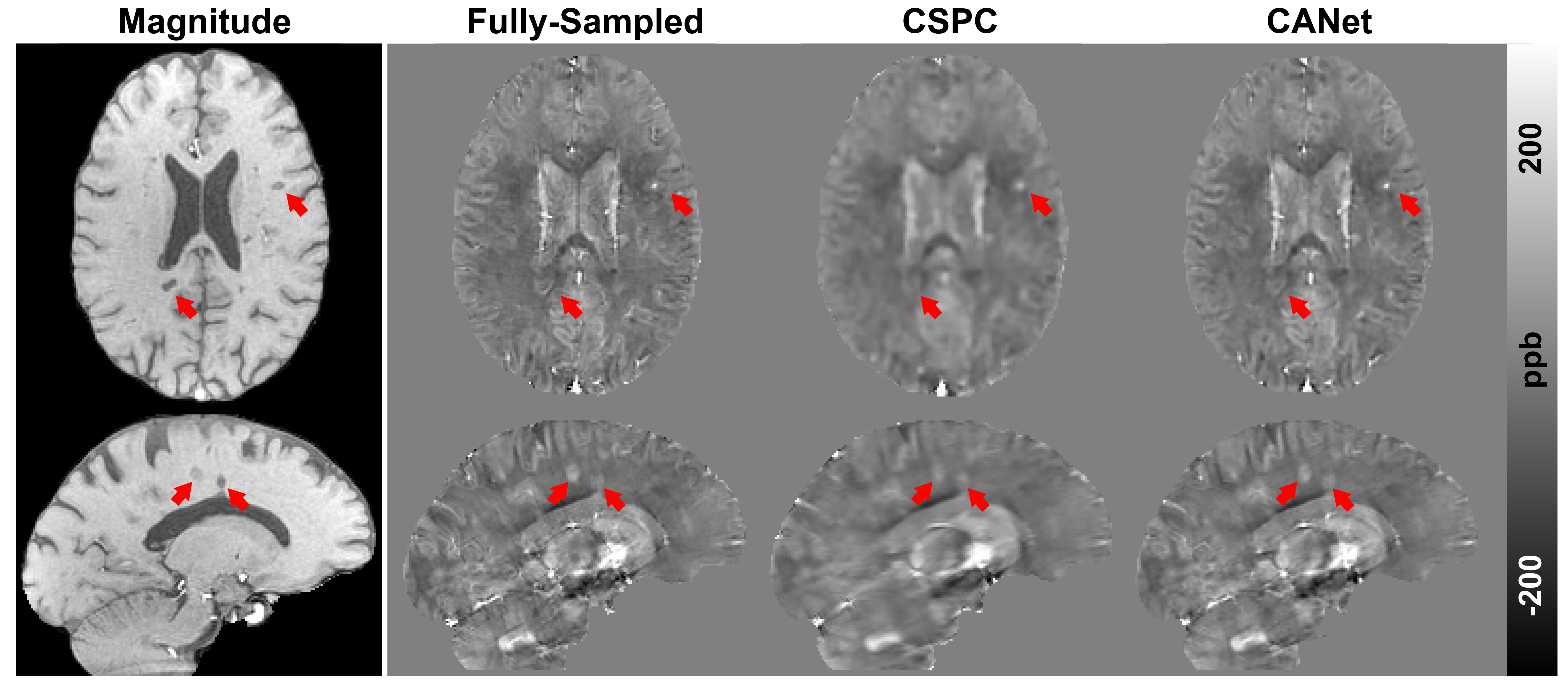
The results from an MS subject are shown in Figure 5. All QSM acceleration methods successfully detected all the brain lesions, as indicated by the red arrows. However, the CSPC method led to significant over-smoothing effects, which is negligible in the reconstructions from CANet.

Discussion and Conclusion

In this study, we proposed a deep network-based MRI reconstruction method (i.e., CANet) to accelerate phase-based QSM, which led to fewer reconstruction errors and more accurate susceptibility estimations than the state-of-the-art CSPC method. The improvement may be due to the reason that conventional regularizers used in CSPC (e.g., wavelet transform) tend to over-smooth the MRI reconstruction, while deep learning method can learn more effective regularizers from the training datasets, which reduces the image over-smoothing.

Acknowledgements

No acknowledgement found.