0735
Neural network-based cr-EPT stabilization.1Medical Engineering, Chiba University, Chiba, Japan, 2Department of Surgery, National University of Singapore, Singapore, Singapore, 3Engineering Product Development, Singapore University of Technology and Design, Singapore, Singapore, 4Artificial Intelligence Research Center, National Institute of Advanced Industrial Science and Technology, Tokyo, Japan, 5Center for Frontier Medical Engineering, Chiba University, Chiba, Japan
Synopsis
Electrical properties are a novel contrast mechanism for quantitative MRI. Conductivity can be used as a biomarker for tumorous tissues. Different analytic Magnetic-Resonance Electrical Properties Tomography (MREPT) methods have been proposed, however, accurate reconstructions require empirical assessment and setting of regularization coefficients per sample. In this work, based on a modified formulation of Convection-Reaction Equation-Based EPT (cr-EPT), the regularization coefficients are learned from the difference between reconstructed conductivity maps and their ground truth, using a convolutional neural network (CNN) model. The CNN model with the modified cr-EPT could achieve conductivity reconstructions with higher accuracy, compared to several analytical models.
Introduction
Magnetic resonance electrical properties tomography (MREPT)1 is a non-invasive technique to obtain conductivity maps from MRI $$$B_1$$$ (RF field) measurements based on the Maxwell equations. Conductivity can be used as a biomarker for tumorous tissues2,3. However, most methods of MREPT methods suffer from noise sensitivity due to the derivatives of $$$B_1$$$ in the formulation4. Even in low-noise cases, most analytical MREPT methods suffer from regularization complexity. There are two types of regularization required for accurate reconstruction: i) a diffusion coefficient that smooths the solution to avoid artifacts from numerical inaccuracies5, ii) an additional convection coefficient which improves the reconstruction accuracy6. Therefore, to reconstruct a conductivity map, one approach is to solve the modified Convection-Reaction Equation based EPT (cr-EPT) in Eq. (1)6. $$\bf{β}(∇φ^{tr} ∇γ)+∇^2 φ^{tr} γ-\bf{ρ}∇^2 γ=ωμ_0\;\;\;\;\;\;\;\;\;\;\;\;\;(1)$$where $$$φ^{tr}$$$ is the transceive phase from the $$$B_1$$$ field, $$$γ$$$ is the inverse of the conductivity $$$1/σ$$$, $$$ω$$$ is the Larmor frequency, $$$\bf{ρ}$$$ is the diffusion coefficient, and $$$\bf{β}$$$ is the convection coefficient. In our previous works7, we showed that local diffusion coefficients improve the accuracy of the reconstructions. Moreover, we proposed a framework for learning the regularization coefficients from the difference between reconstructed conductivity maps and their ground truth, by a neural network8. The framework was tested with simple samples, and preliminary results were shown. In this work, the framework was further tested with one multiple-cylinder sample set and another digital human brain sample set.
Methods
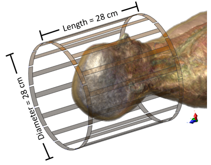
Fig. 1 shows the framework of the proposed Neural network-based cr-EPT stabilization where a neural network was trained to learn to produce both local diffusion ($$$\bf{ρ}$$$) and convection coefficients ($$$\bf{β}$$$), by considering the $$$φ^{tr}$$$ measurement and its derivatives (Inputs). We solve the cartesian discretized modified cr-EPT (1) equation every epoch for the training samples in Pytorch©9, a neural network framework to capitalize from automatic differentiation. The structural similarity index measure (SSIM) difference is feedbacked through the gradient of the operations of the modified cr-EPT by automatic differentiation (backpropagation) to improve the regularization coefficients. Thus, the neural network learns to produce accurate local regularization coefficients. SSIM is selected as the loss function to avoid diffused reconstructions. A five-layer convolutional neural network (CNN) is chosen due to its high efficiency on images and low memory cost. The regularization coefficients need to be constrained to avoid taking over the equation. To constraint the values of the coefficients, the coefficients are squeezed by a sigmoid function multiplied by the maximum value of the coefficient $$$(β_{max}=4,ρ_{max}=0.1)$$$. The boundaries of the regularization coefficients are selected empirically. The network is trained for 1000 epochs and optimized via ADAM10.We produced various numerical simulations in Sim4Life© to create two small datasets, one from the ELLA anatomical model11 (8 samples for training, 2 samples for testing) and another for a multi-cylinder model (8 samples for training, 2 samples for testing). A high-pass 16 rung 3T MRI coil of 14 cm radius and 28 cm in length is created in the simulation environment. The coil is excited in quadrature mode, to increase $$$B_1$$$ homogeneity and reduce artifacts on the reconstruction. The coil is loaded with the structures to be reconstructed, as can be seen in Fig. 2.
Results
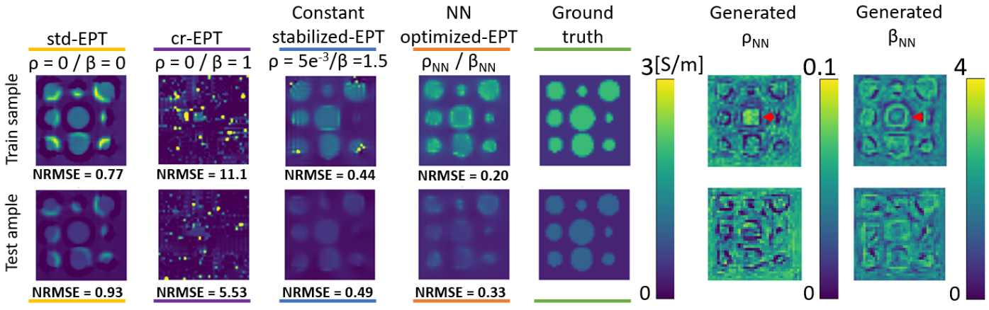
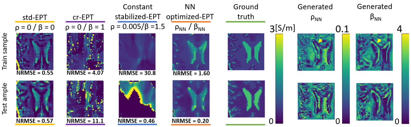
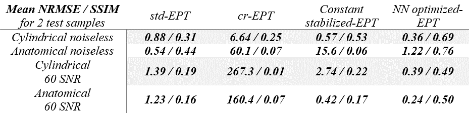
One test and one train samples reconstruction are shown in Fig. 3 for the multiple-cylinder model dataset, with the learned regularization coefficients, independent comparison with std-EPT $$$(β=0,ρ=0)$$$, cr-MREPT $$$(β=1,ρ=0)$$$ and homogeneously stabilized cr-EPT $$$(β=1.5,ρ=5e^{-3})$$$ reconstruction are shown. NRMSE is shown as an accuracy metric. For the digital human model dataset, the reconstruction for a train and a test sample is also shown as a feasibility test in Fig. 4. Fig. 5 shows a comparative table with results for the multiple-cylinder and digital human test samples from the reconstruction methods for noiseless and noisy cases.Discussion
CNN-based coefficient selections provide higher accuracy reconstructions. The noise response of the method is robust. However, since derivative calculations are not modified, noise-related artifacts are still present in the reconstruction. Future work will be focused on improving the derivative calculation of the $$$φ^{tr}$$$ to reduce noise-related artifacts. This method can be used to produce permittivity reconstructions as well. The method could be exploited to extract the information learned by the network to produce general rules of the coefficients for any samples. The two regularization coefficients appear to work complementarily, which can be observed in the boundary area indicated by red arrows in generated $$$\bf{ρ}$$$ and generated $$$\bf{β}$$$ maps in Fig. 3. High $$$\bf{ρ}$$$ values resulted in diffused on the corresponding area in the reconstructed conductivity map, and high $$$\bf{β}$$$ values enforced the boundary. Similar behavior can be observed for the complex human head model, as shown in the boundary area indicated by yellow arrows in Fig. 4. However, further analysis is necessary. The model could generalize the coefficient selection, even with a low number of samples, likely due to the physical constraints the model enforces on the CNN.Conclusion
In this work, we showed that local regularization coefficients from a modified cr-MREPT model can be learned by a CNN from the difference between reconstructed conductivity maps and their ground truth. The local coefficients from CNN increased the accuracy of the conductivity reconstructions.Acknowledgements
No acknowledgement found.References
1. Katscher U, Findeklee C, Vernickel P, Nehrke K, Voigt T, Dössel O. Determination of Electric Conductivity and Local SAR Via B1 Mapping. IEEE Trans Med Imaging. 2009;28(9):1365-1374. doi:10.1109/TMI.2009.2015757
2. Tha KK, Katscher U, Yamaguchi S, et al. Noninvasive electrical conductivity measurement by MRI: a test of its validity and the electrical conductivity characteristics of glioma. Eur Radiol. 2018;28(1):348-355. doi:10.1007/s00330-017-4942-5
3. Mori N, Tsuchiya K, Sheth D, et al. Diagnostic value of electric properties tomography (EPT) for differentiating benign from malignant breast lesions: comparison with standard dynamic contrast-enhanced MRI. Eur Radiol. 2019;29(4):1778-1786. doi:10.1007/s00330-018-5708-4
4. Mandija S, Sbrizzi A, Katscher U, Luijten PR, van den Berg CAT. Error analysis of Helmholtz-based MR-electrical properties tomography. Magn Reson Med. 2018;80(1):90-100. doi:10.1002/mrm.27004
5. Li C, Yu W, Huang SY. An MR-Based Viscosity-Type Regularization Method for Electrical Property Tomography. Tomogr (Ann Arbor, Mich). 2017;3(1):50-59. doi:10.18383/j.tom.2016.00283
6. Ider YZ, Akyer MN. Properties and implementation issues of phase-based cr-MRECT for conductivity imaging. In: Proc. Intl. Soc. Mag. Reson. Med. 28. 2020:3190.
7. Garcia AJ, Huang S, Yu W. Region-specific regularization of convection-reaction Magnetic Resonance Electrical Property Tomography ( MREPT ) for improving the accuracy and noise-tolerance of EP reconstruction. In: Proc. Intl. Soc. Mag. Reson. Med. 26. 2018:2286.
8. Garcia A, Huang SY, Imamoglu N, Yu W. Machine-learning-enhanced stabilized cr-MREPT for noise-robust and artifact-reduced electrical properties reconstruction. In: Proceedings 2020 IEEE International Conference on Computational Electromagnetics (ICCEM2020). 2020:130-132.
9. Paszke A, Gross S, Massa F, et al. PyTorch: An imperative style, high-performance deep learning library. Adv Neural Inf Process Syst. 2019;32.
10. Kingma DP, Ba JL. Adam: A method for stochastic optimization. 3rd Int Conf Learn Represent ICLR 2015 - Conf Track Proc. 2015:1-15.
11. Gosselin M-C, Neufeld E, Moser H, et al. Development of a new generation of high-resolution anatomical models for medical device evaluation: the Virtual Population 3.0. Phys Med Biol. 2014;59(18):5287-5303. doi:10.1088/0031-9155/59/18/5287Figures
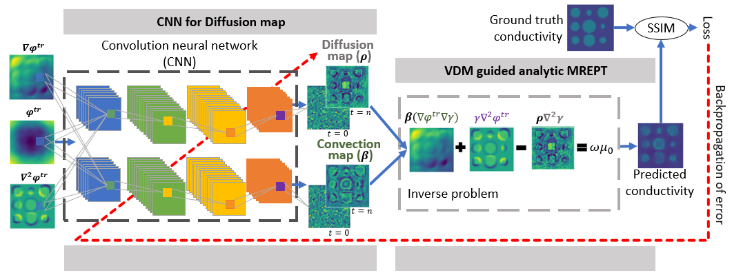
Figure 1. Structure of the framework. The CNN receives $$$φ^{tr}$$$ maps and their derivatives as inputs. The CNN produces the local regularization coefficients, which are used to solve the inverse problem. The error between the predicted conductivity map and their ground-truth is backpropagated to the CNN to update the parameters.