Introduction

A major caveat of acquisitions with long readout durations are artifacts introduced by B₀ inhomogeneity. These artifacts can be addressed in image reconstruction when incorporating a field map¹. However, acquiring these maps requires an additional scan and the validity of the maps can change over the course of an MR scan due to heating of the MR system or motion of the volunteer. Hence, it is an intriguing option to obtain B₀ from the acquired dataset itself. This goal has been pursued with EPI blip up/down² or spiral-in/out³ acquisitions. However, these approaches still require multiple acquisitions of the same k-space portion.
In this work, we propose field estimation and correction based on generic single acquisitions, exploiting implicit B₀ encoding by array detection. Standard EPI and spiral-out in-vivo scans of undersampling factors up to$$$\;R=4\;$$$are corrected using the proposed method requiring no initial information on B₀.

Methods

Cost Function
Given the measured signal$$$\;\mathbf{m}\;$$$the joint reconstruction of the discretized object$$$\;\mathbf{v}\;$$$and field map$$$\;\mathbf{\Delta\omega_0}\;$$$can be conceived as minimization of the loss
$$\mathcal{L}(\mathbf{\Delta\omega_0},\mathbf{v})=\Vert\mathbf{m}-E(\mathbf{\Delta\omega_0})\mathbf{v}\Vert^2.\;\;\;\;\;(1)$$.
Here,$$$\;E\;$$$denotes the encoding matrix^4,5 incorporating$$$\;\mathbf{\Delta\omega_0}\;$$$
$$E_{(\sigma,\kappa),\rho}=s_\sigma(\textbf{r}_\rho)e^{i\textbf{k}(t_\kappa)\cdot\textbf{r}_\rho}e^{i\Delta\omega_0(\textbf{r}_\rho)t_\kappa}\;\;\;\;\;(2)$$with the voxel position $$$\mathbf{r}_\rho$$$, coil sensitivities$$$\;s_\sigma$$$, k-space trajectory$$$\;\textbf{k}_\kappa\;$$$and their respective discretization indices$$$\;\rho,\sigma,\kappa$$$. The number of unknowns can be vastly reduced by limiting the search space to only those objects that minimize$$$\;\mathcal{L}\;$$$for any given$$$\;\mathbf{\Delta\omega_0}$$$:$$\mathbf{v}=E^+(\mathbf{\Delta\omega_0})\mathbf{m}.\;\;\;\;\;(3)$$Inserting Eq. (3) into (1) yields a cost function solely depending on the unknown field map$$$\;\mathbf{\Delta\omega_0}$$$:$$\mathcal{L}(\mathbf{\Delta\omega_0})=\Vert(\text{Id}-E(\mathbf{\Delta\omega_0})E^+(\mathbf{\Delta\omega_0}))\mathbf{m}\Vert^2.\;\;\;\;\;(4)$$Note that no assumption on the used trajectory or coil set-up is made.

Regularization
Since not all possible configurations of$$$\;\mathbf{\Delta\omega_0}\;$$$are physically reasonable, a regularising basis incorporating this a-priori knowledge is chosen. In this work, field offsets are modelled by 2D Gaussian basis functions$$$\;\beta\;$$$defined on a sparse grid$$$\;\mathbf{r}_i\;(\sigma_{Gauss}=0.5\;$$$grid-units)⁶$$\Delta\omega_0(\mathbf{r})\approx\sum_ib_i\mathbf{\beta}_i.\;\;\;\;\;(5)$$Inserting this into Eq. (4), the loss becomes a function of the coefficients$$$\;b_i\;$$$with a reduced number of unknowns.

Optimization
The analytic derivative of the loss (Eq. (5) inserted into Eq. (4)) with respect to$$$\;\mathbf{b}\;$$$is given by$$\frac{\partial\mathcal{L}(\mathbf{b})}{\partial\,b_i}=2\text{Re}\{-i\;\text{diag}((E(\mathbf{b})^+\mathbf{m})^H)E(\mathbf{b})^H\text{diag}(\mathbf{t})(\mathbf{m}-E(\mathbf{b})(E(\mathbf{b})^+\mathbf{m}))\}\cdot\mathbf{\beta}_i.\;\;\;\;\;(6)$$To find the optimal field map estimate, i.e. minimizing the loss$$$\;\mathcal{L}$$$, a gradient descent method is performed until convergence. Each evaluation of the loss$$$\;\mathcal{L}(\mathbf{\Delta\omega_0})\;$$$includes an image reconstruction (Eq. (3)) which is done iteratively using the CG-method⁵ to reduce computation time.

Implicit B0 Encoding
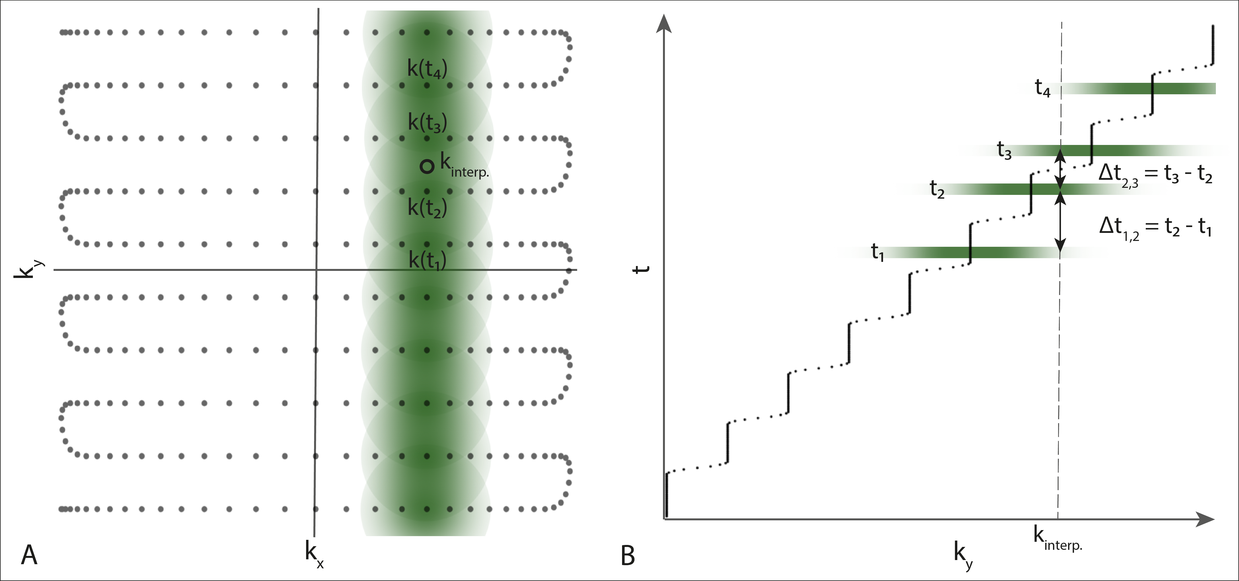
Trying to solve for B₀ in this fashion using mono-acquisitions rests on the hypothesis that array detection performs implicit B₀ encoding. The coil array allows for extrapolation in k-space as used extensively in parallel imaging, see Fig. 1A. The extrapolation by the coil-array viewed in k-t space, Fig. 1B, shows that information about most measurement samples is also given at different times leading to a temporal encoding.
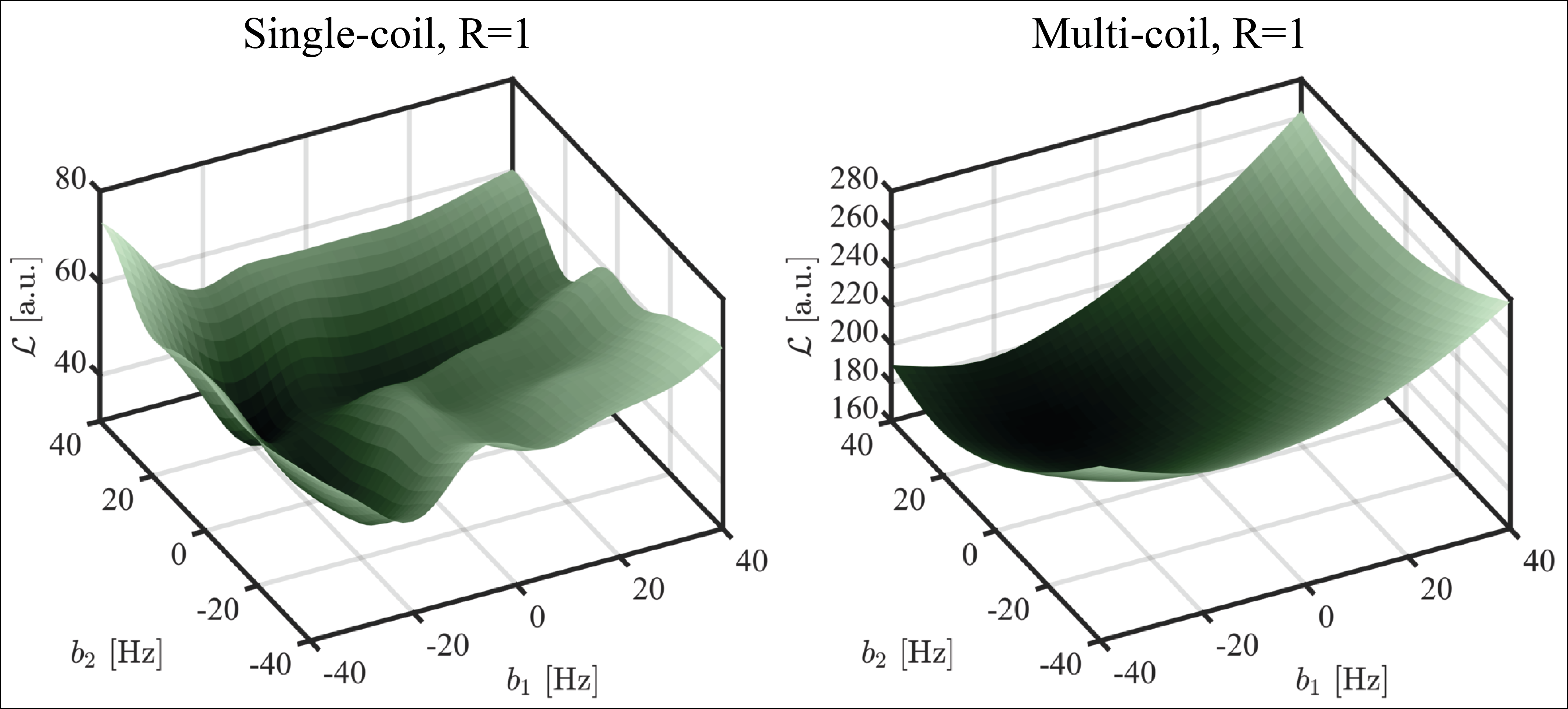
To investigate this mechanism and its influence on the cost, a field map modelled by two Gaussian basis functions was simulated and the cost$$$\;\mathcal{L}\;$$$was determined on a grid for a single- and multi-coil setup.

Data acquisition
Data was acquired on a 3T MR system (Philips Healthc­­are, Best, The Netherlands) using a 16-channel head coil with integrated magnetic field sensors⁷ (Skope MR Technologies, Zurich, Switzerland). EPI scans were acquired with$$$\;2.2^2,1.4^2,1.1^2mm^2\;$$$for$$$\;R=1,2,3\;$$$and spiral-out scans with$$$\;1.7^2,1.1^2,0.9^2,0.8^2mm^2\;$$$for$$$\;R=1,2,3,4$$$,$$$\;\text{TE}=25ms$$$,$$$\;\text{FOV}=24x24cm$$$. Additionally, a two-echo GRE sequence$$$\;(\Delta\,t=2.4ms)\;$$$was acquired to fit a field map for reference.

Results

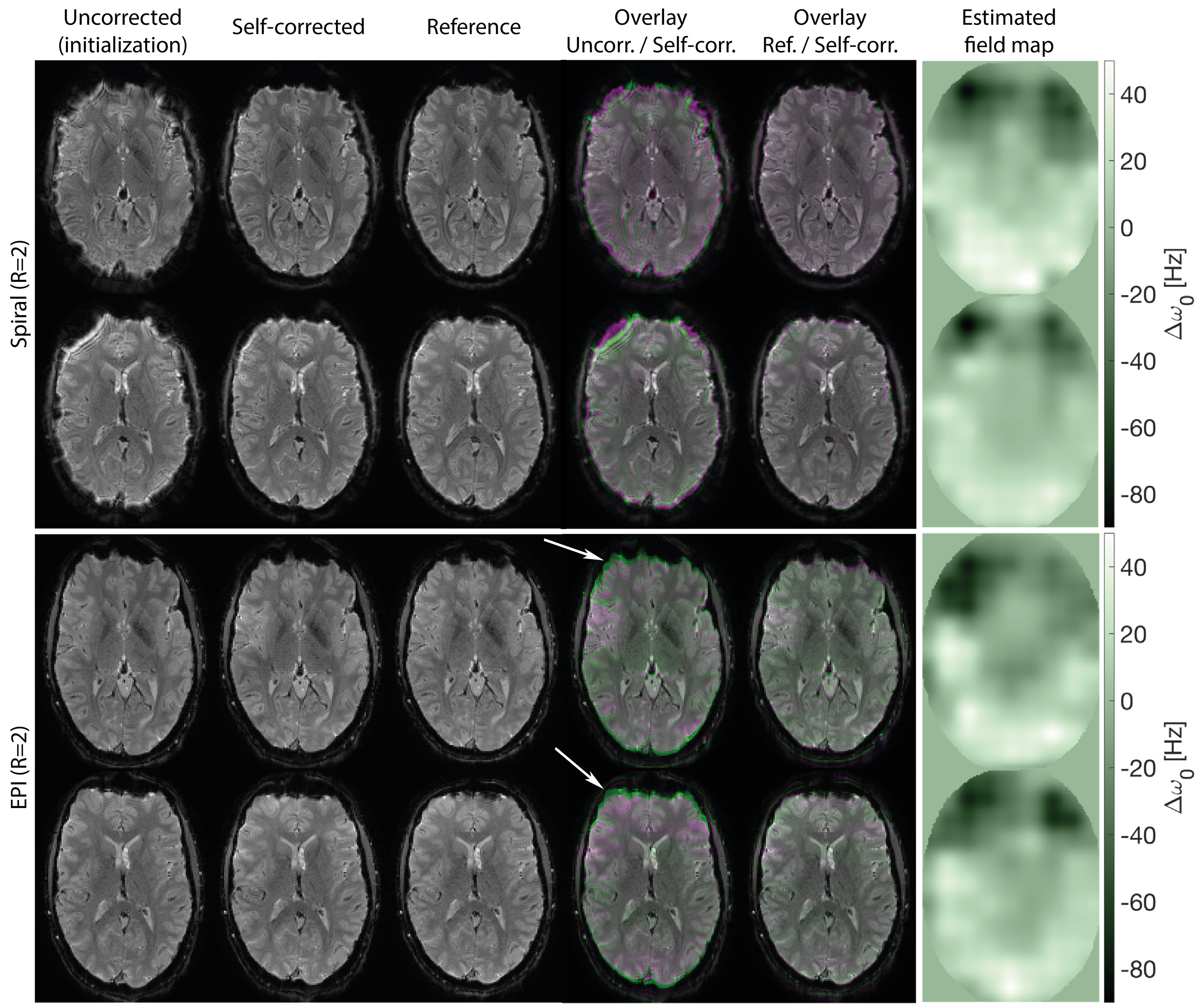
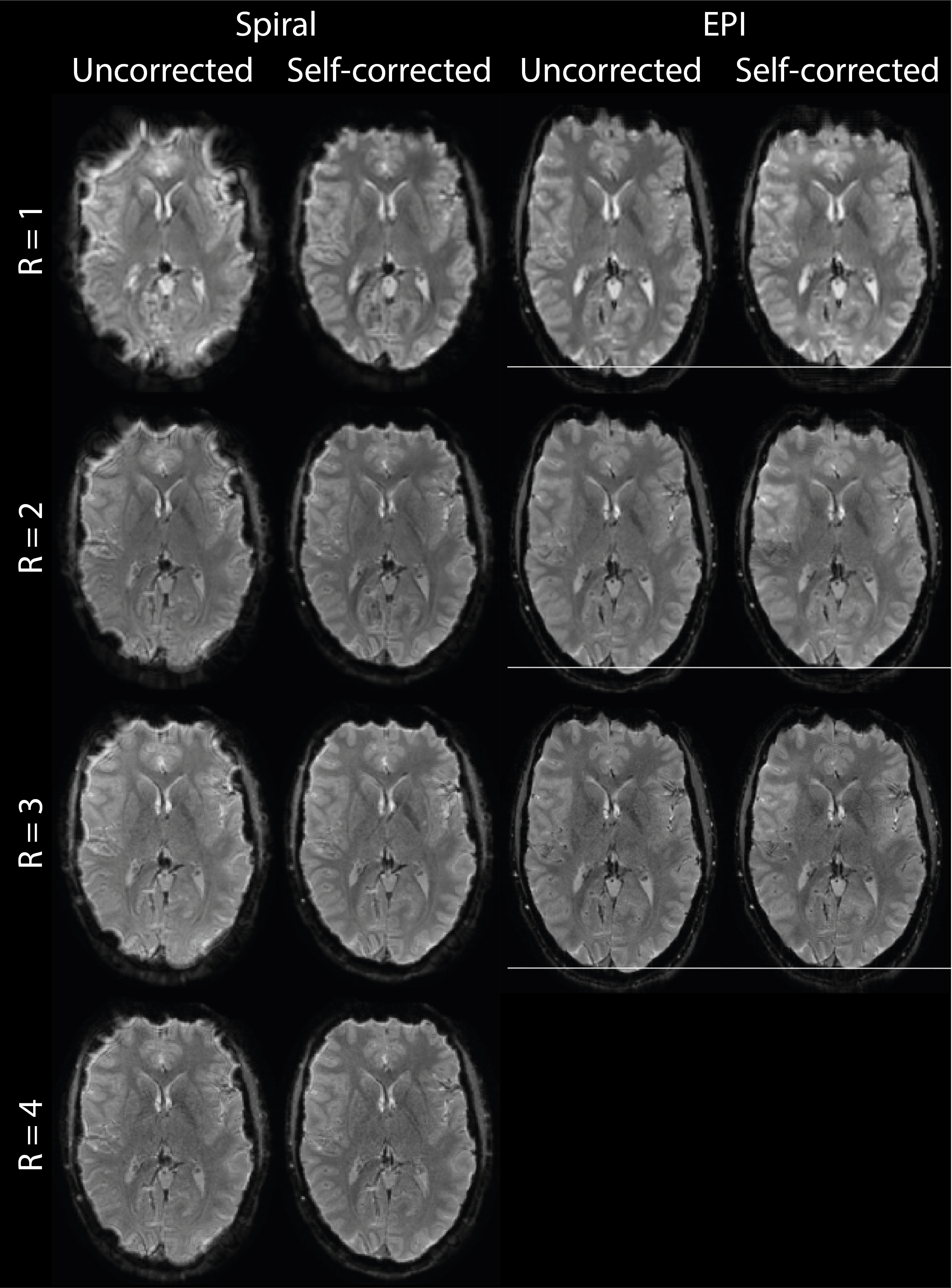
The cost landscape of the single-coil set-up exhibits several local minima on the covered search space whereas in the multi-coil set-up only one local minimum at the right location is visible (Fig. 2). This indicates that (a) the multi-coil set-up is capable of encoding temporal information and (b) attractor sizes seem to be large enough to start the optimization with no information on B₀.
Initializing with the uncorrected distorted images, i.e.$$$\;\mathbf{\Delta\omega_0}=\mathbf{0}$$$, the algorithm converged towards images with strongly reduced blurring (spirals) and geometric distortions (EPI) as well as a bigger agreement to the reference images obtained from a reconstruction using the reference field map (Fig. 3). The estimated field maps modelled by$$$\;13\times13\;$$$basis coefficients were similar for EPI and spiral acquisitions in both slices.
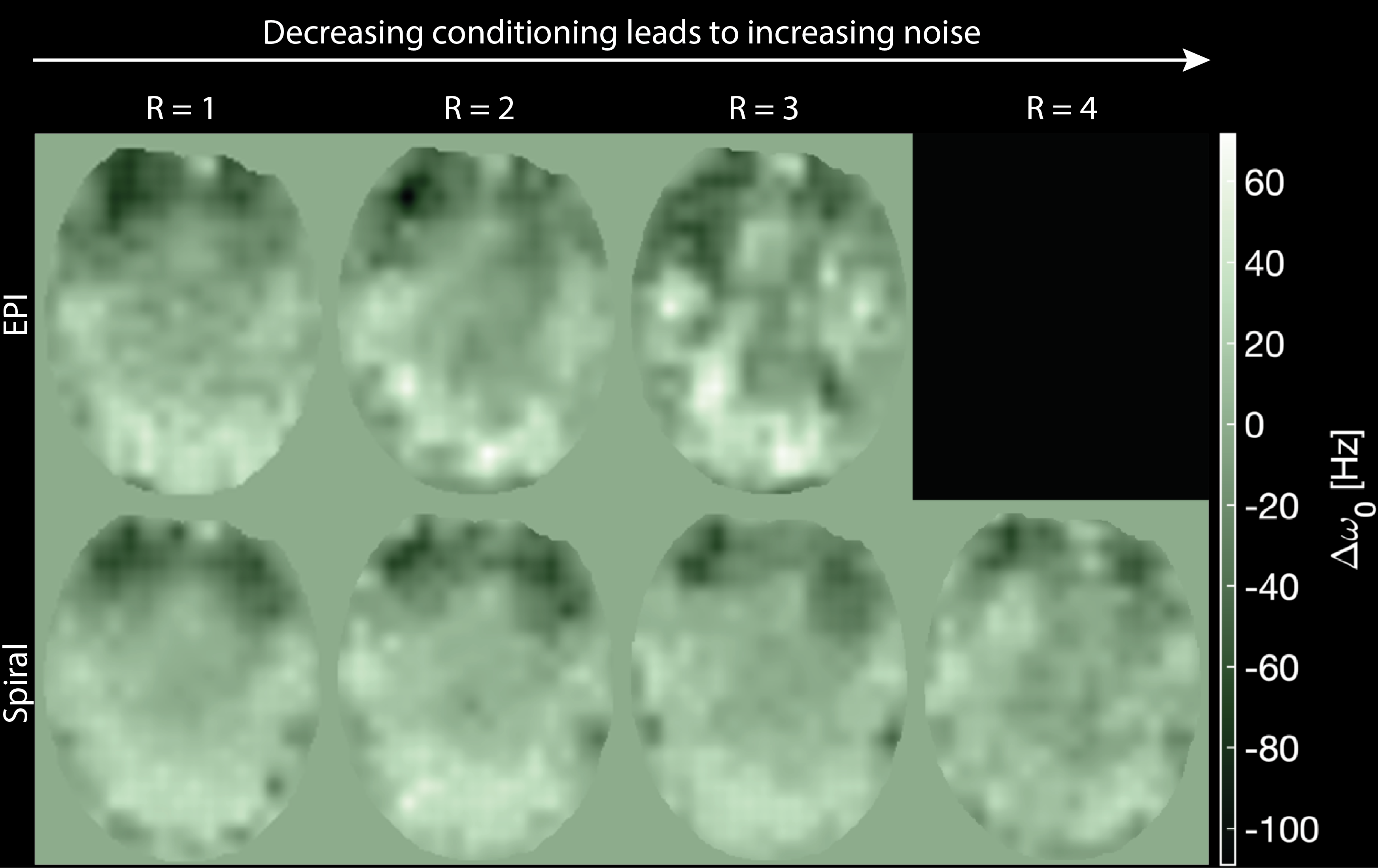
The capability of the array to encode temporal information, i.e. the conditioning of the B_0-estimation problem, decreases with an increasing acceleration factor$$$\;R\;$$$and depends on the used trajectory (Fig. 4). The field maps obtained from spiral images show less noise and indicate a better conditioning presumably owing to the less-coherent encoding pattern (Fig. 4). The number of basis coefficients, i.e. the regularization of the problem, may be adjusted to allow more robust (albeit less accurate) B₀-estimation and correction for images acquired with higher undersampling factors (Fig. 5).

Discussion and Conclusion

The feasibility of B₀-estimation without relying on multiple k-space acquisitions even for highly undersampled data was demonstrated.
B₀ self-correction appears to be harder when the distortions are wide-ranging compared to the FOV ($$$R=1\;$$$cases Fig. 5) as the information on B₀ is spread further away from its origin. Highly accelerated data showed as expected a worse conditioning but was still good enough to lead to strongly improved images (R=3,4 Fig. 5).
The method can directly benefit several applications that typically rely on single-shot imaging such as fMRI or DWI/DTI, but may also be used for multi-shot acquisitions for structural imaging⁸ that use long (SNR efficient) readouts.
The proposed method also raises several new questions. On the hardware side, the B₀-encoding capabilities of different arrays may be investigated. Moreover, the effect of trajectory design (e.g. using variable density acquisitions) may be further studied.

Acknowledgements

The authors would like to thank Yoojin Lee and Simon Gross.