Introduction

Cardiac-related hemodynamic pulsatility in the brain is associated with upstream central artery stiffening, an important characteristic of cerebrovascular disease.¹ Elevated pulsatility in conduit intracranial arteries, such as the middle cerebral artery, is thought to contribute to microvasculature damage in brain tissue. Such vascular information is contained within the BOLD signal and, conventionally, has been isolated only by retrospectively sorting BOLD data based on a corresponding cardiac trace.^2,3,4 Many neuro-MRI studies, however, do not record the cardiac trace, prohibiting voxelwise assessment of cardiac-related pulsatile contributions to the BOLD signal. The current study attempts to alleviate the need for cardiac recordings by training a convolutional neural network to identify these features in BOLD data and generate estimates of brain pulsatility.

Methods

Scans were collected from 43 healthy adults (11 young and 32 older adults). Imaging was performed on a 3T MRI (Achieva, Philips Healthcare) with an 8-channel head coil receiver. The protocol included high-resolution T1-weighted (T1w) 3D imaging (TR/TE=9.5/2.3 ms, flip angle = 8º, voxel size = 0.630.631.2 mm, 140 axial slices) and multi-echo T2*-weighted echo planar imaging (TR=2300 ms, TE1/TE2/TE3=13.82/35.35/56.89 ms, flip angle = 70º, voxel size = 2.882.884 mm, 28 axial slices, 195 volumes). In this work, we used only the data acquired with TE2, hereafter referred to as the BOLD data. During scanning, a pulse oximeter collected the cardiac trace and respiratory bellows recorded the respiration trace.

Ground truth pulsatility maps, used for network training, were estimated from the BOLD data by regressing out respiratory influences⁵, sorting volumes by their temporal position within the cardiac cycle, and fitting a 7-term Fourier series to the sorted data. The degree of pulsatility in a voxel was calculated as the normalized root mean square of the Fourier series coefficients. Therefore, pulsatility maps are unitless and expressed as Z-scores (standard deviations from mean). Additional methods details are described previously.^3,4

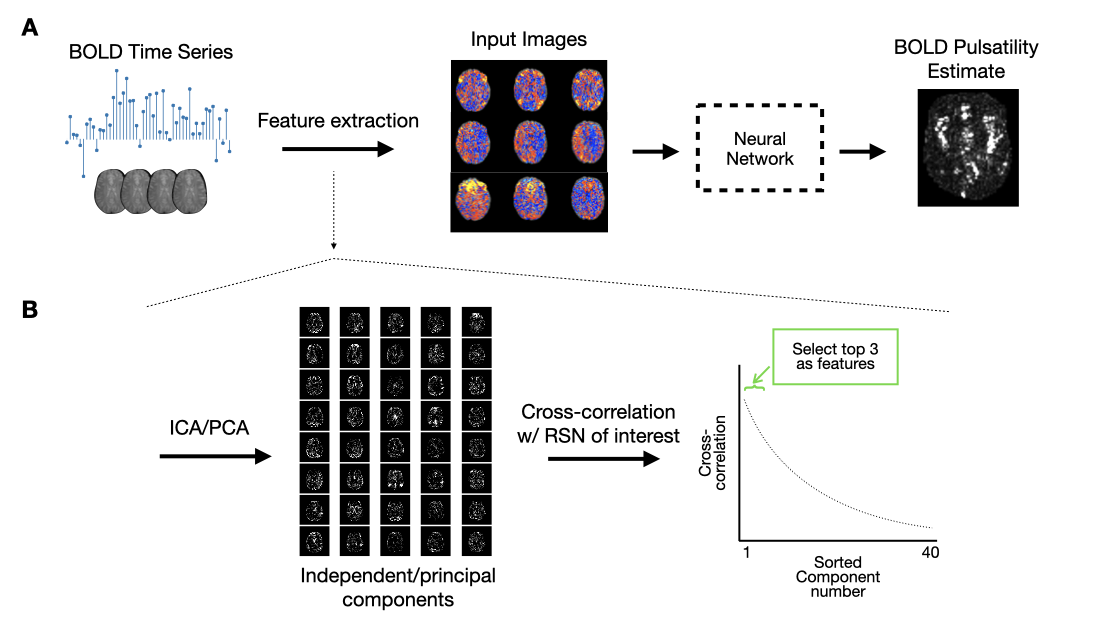
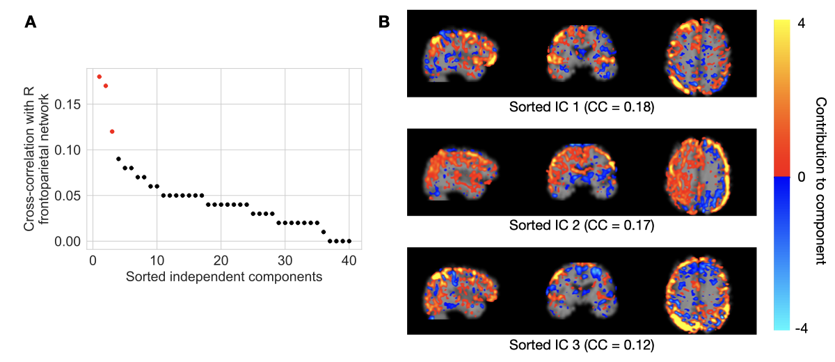
Processed BOLD images were used as inputs to the neural network (Figure 1). Three separate dimension reduction approaches were considered: independent component analysis (ICA), principal component analysis (PCA), and the Fourier transform. In each of the two component analyses, forty components were computed. Nine total components were selected as network inputs based on spatial correlation with three pre-defined resting-state networks; we chose the executive-control network and the bilateral frontal-parietal networks, a priori, due to their spatial overlap with areas of conduit artery pulsatility. In the Fourier analysis, the first nine terms of the transformed BOLD signal were selected as inputs.

We trained a 2D convolutional neural network based on a U-Net architecture to estimate pulsatility in each image slice (trained on a NVIDIA P100 Pascal GPU). The training set was constructed by randomly selecting 80% of the 43 scans. Eight epochs and a five-fold cross-validation on the training set (i.e. all slices from 34 scans) were used to select the best-performing input features between the ICA-, PCA-, and Fourier-based inputs. The network was re-trained for fifteen epochs on all training data and performance was assessed on the remaining 20% of data. Performance was based on whole-brain mean absolute error between network estimates and ground truth.

Results

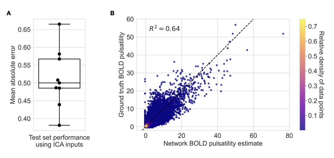
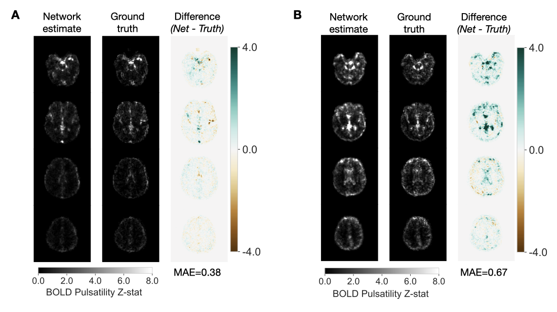
Representative results from the feature selection process are shown in Figure 2. The network trained using ICA-based inputs had the lowest mean absolute error of 0.601±0.102 in estimating the (unitless) voxelwise pulsatility Z-scores. The networks trained using PCA-based and Fourier transform-based inputs had mean absolute errors of 0.637±0.117 and 0.603±0.114, respectively.

After re-training on ICA-based inputs from all data used for cross-validation, the average network error on scans in the test set was 0.513±0.083 (Figure 3A). Network estimates were able to explain 64 percent of the variance in ground truth pulsatility, on a voxelwise basis (Figure 3B). Best and worst mean absolute error for test cases are shown in Figure 4.

Discussion

We trained a convolutional neural network to estimate cardiac-related hemodynamic pulsatility using data-driven, dimensionality-reduced, BOLD-based features. This proof-of-concept study demonstrates the feasibility of generating BOLD pulsatility maps without a reference cardiac trace. This method enables the study of downstream effects of arterial stiffening, and therefore cerebrovascular disease, in a wider range of retrospective and future studies.

Cross-validation revealed the network performed best when trained on ICA-based inputs, although mean absolute errors from the three input types were comparable. Near large arteries, where pulsatility is highest, a large fraction of BOLD signal variance is explained by the cardiac cycle;6 therefore, it is unsurprising that any of the dimensionality reduction techniques, which capture the majority of signal variance, have similar utility in estimating pulsatility.

The network performed better during testing compared to cross-validation, likely due to more training epochs and more training data (all data rather than the training set of a single fold). In the test data, the neural network model captured the majority of variance in ground truth pulsatility. The model correctly estimated high pulsatility in regions near large intracranial arteries, although errors tended to increase as pulsatility increased. Future work will therefore focus on improving estimates in these regions, such as the insular cortex, in which pulsatility is known to correlate with direct arterial measurements of pulsatile flow.⁴

Acknowledgements

No acknowledgement found.