0612
Improved Slice Coverage in Inversion Recovery Radial Balanced-SSFP using Deep Learning
Eze Ahanonu1, Zhiyang Fu1,2, Kevin Johnson2, Maria Altbach2,3, and Ali Bilgin1,2,3
1Electrical and Computer Engineering, University of Arizona, Tucson, AZ, United States, 2Medical Imaging, University of Arizona, Tucson, AZ, United States, 3Biomedical Engineering, University of Arizona, Tucson, AZ, United States
1Electrical and Computer Engineering, University of Arizona, Tucson, AZ, United States, 2Medical Imaging, University of Arizona, Tucson, AZ, United States, 3Biomedical Engineering, University of Arizona, Tucson, AZ, United States
Synopsis
Abdominal T1 mapping is important for quantitative evaluation of various pathologies. A recent inversion recovery radial balanced-SSFP (IR-radSSFP) technique allows high resolution T1 mapping of ten slices within a single breath hold period (BHP), but requires multiple BHPs for full abdominal coverage. We propose an accelerated T1 mapping framework which utilizes deep learning to estimate T1 using a fraction of the T1 recovery curve (T1RC). In vivo experiments demonstrate that the proposed framework achieves less than 6% T1 error while using only 25% of the T1RC of the earlier IR-radSSFP technique. This enables full abdominal coverage within a single BHP.
Introduction
T1 mapping of the abdomen has been demonstrated to be useful for quantitative evaluation of various pathologies.1,2 Recently, rapid 2D radial Look Locker techniques were proposed for multi-slice high resolution T1 mapping of the abdomen.3,4 These techniques allow for the acquisition ~10 high-resolution slices within a single breath hold period (BHP) and therefore require multiple BHPs for full abdominal coverage. Deep-learning (DL) techniques have been proposed for MR relaxometry applications.5,6 These DL techniques exploit the spatio-temporal redundancies to improve T1 estimation performance. In this study, we propose a DL approach to improve the slice coverage of 2D radial Look Locker methods.Methods
Figure 1 summarizes the radial 2D Look Locker T1-mapping technique (inversion recovery radial steady-state free precession (IR-radSSFP)).1 Let $$$T_{S}$$$ and $$$S$$$ represent the acquisition time for one slice and the number of acquired slices, respectively. The radial views acquired throughout the T1 recovery curve (T1RC) for each slice are grouped into N inversion time (TI) groups from which N TI images are reconstructed. Data acquisition for all acquired slices need to be completed within the BHP time $$$T_{BHP}$$$: $$$S\cdot T_{S}\leq T_{BHP}$$$. Therefore, to accommodate more slices, the acquisition time per slice $$$T_{S}$$$ needs to be reduced. If the $$$T_{S}$$$ is reduced substantially (e.g. less than 2 seconds) by reducing N, the T1 relaxation time cannot be estimated accurately using conventional nonlinear least squares (NLLS) curve fitting,7 especially for long T1 species. We note, however, that the T1 signal evolves rapidly during early recovery and slows in the later recovery regime (Figure 1.a). Thus, we propose a strategy where the number of TIs along the T1RC is reduced but T1 estimation is performed using a convolutional neural network (CNN), which exploits the spatio-temporal redundancies in T1RC to improve T1 estimation performance.The proposed DL framework is presented in Figure 2. The inputs to our DL model ($$$X=\{{I_{1},...,I_{\hat{N}}}\}$$$) are a set of TI images which have undergone iterative reconstruction, where $$$\hat{N}\leq N$$$ indicates a reduced number of TIs. The output of our model $$$\hat{T}_{1}$$$ is an estimate of the T1 map. The network targets/labels are T1 maps obtained using N TI images.
Ten subjects were imaged using the 2D IR-radSSFP sequence with TR=4.40ms, TE=2.15ms, 32 TIs, in-plane resolution=0.83mmX0.83mm, slice thickness=3mm, 10 slices, and 16 lines/TI with 384 readout points/line. Reference T1 maps were obtained using a model-based CS approach8 followed by reduced dimension NLLS curve fitting.7 These full T1RC datasets were retrospectively undersampled by selecting the first $$$\hat{N}=8,12,16,20,24,28$$$ TI groups. Similarly, the TI images at different number of truncations were individually reconstructed using the CS approach. For each $$$\hat{N}$$$, a neural network is trained using $$$\hat{N}$$$ TI images as inputs and the corresponding reference T1 maps obtained with $$$N=32$$$ as targets. We used ResNet9 as the backbone of our network consisting of 16 residual blocks, where each block contains two 32-filter convolutional layers with batch normalization. The network was trained for 100 epochs using a fixed learning rate of 1e-4 and an L2 weight decay of 1e-4. Patch extraction (16x16) as well as random rotation and flip were applied for data augmentation. In each experiment, 7 subjects were randomly selected for training, 2 subjects were randomly selected for testing. One subject with liver pathology was reserved for testing. ROI analysis of estimated T1 values was performed for NLLS curve fitting and DL methods for each $$$\hat{N}$$$ and compared to reference T1 values.
Results and Discussion
Figure 3 demonstrates performance of the NLLS method when a varying number of TIs are used in estimation. We observe that T1 estimation performance deteriorates significantly in regions where signal-to-noise ratio (SNR) is low, due to poor curve fitting, resulting in substantial variation in T1 estimates between neighboring pixels . Figure 4 provides a comparison of T1 estimations using NLLS and the proposed DL framework. Nine ROIs (with varying noise levels and tissue types) from three slices were used to evaluate the T1 mapping performances. The DL model achieved under 2% estimation error (as measured by relative mean absolute error) across all number of TIs ($$$\hat{N}$$$) in lower-noise regions of the liver, whereas the estimation error for NLLS increased sharply below 16 TIs. For the higher-noise liver and spleen regions the DL model estimation error is within 6% across all $$$\hat{N}$$$. In contrast, NLLS yields large estimation errors when $$$\hat{N}$$$ falls below 24. Figure 5 provides an example of T1 values in a subject with a liver lesion using NLLS and DL methods for varying $$$\hat{N}$$$. Within the lesion, the DL model achieved under 6% estimation error up until $$$\hat{N}=16$$$, while for NLLS estimation error exceeded 6% after $$$\hat{N}=28$$$. Figure 5.b provides visual examples of the T1 maps of the lesion ROI, which demonstrate the superior structural integrity of the DL estimated T1 maps across $$$\hat{N}$$$ values.Conclusions
We presented an accelerated T1 mapping framework which utilizes deep learning to extend the slice coverage of 2D radial Look Locker T1 mapping methods. In vivo experiments demonstrate that the proposed method achieves less than 6% T1-estimation error while extending the slice coverage by 4X compared to recent radial Look Locker T1 mapping techniques.Acknowledgements
We would like to acknowledge grant support from NIH (CA245920 and CA245920S1), the Arizona Biomedical Research Commission (ADHS14-082996), and the Technology and Research Initiative Fund Technology and Research Initiative Fund (TRIF).References
- Z Li, A Bilgin, K Johnson, J Galons, S Vedantham, DR Martin, MI Altbach, “Rapid High-Resolution T1 Mapping Using a Highly Accelerated Radial Steady-State Free-Precession Technique,” Journal of Magnetic Resonance Imaging, 49: 239-252, 2018. https://doi.org/10.1002/jmri.26170
- MB Keerthivasan, Z Li, JP Galons, K Johnson, B Kalb, DR Martin, A Bilgin, and MI Altbach, “Characterization of Abdominal Neoplasms using a Fast Inversion Recovery Radial SSFP T1 Mapping Technique,” in Proc. of 2019 Annual Meeting of the ISMRM, Montreal, QC, Canada, May 2019.
- MB Keerthivasan, X Zhong, D Nickel, D Garcia, MI Altbach, B Kiefer, V Deshpande, “Simultaneous T1 and Fat Fraction Quantification using Multi-Echo Radial Look-Locker Imaging,” Proceedings of Annual Meeting of the ISMRM, 28:2478, 2020.
- MB Keerthivasan, D Nickel, F Han, X Zhong, MI Altbach, B Kiefer, V Deshpande, “An Efficient, Robust, and Reproducible Quantitative Radial T1 Mapping Technique,” Proceedings of Annual Meeting of the ISMRM, 28:2478, 3155.
- L Feng, D Ma, F Liu, “Rapid MR Relaxometry Using Deep Learning: An Overview of Current Techniques and Emerging Trends,” NMR in Biomedicine. e4416; 2020. https://doi.org/10.1002/nbm.4416
- Z Fu, S Mandava, MB Keerthivasan, Z Li, K Johnson, DR Martin, MI Altbach, A Bilgin,"A Multi-Scale Residual Network for Accelerated Radial MR Parameter Mapping," Magnetic Resonance Imaging, 73: 152-162,2020.
- JK Barral, E Gudmundson, N Stikov, M Etezadi-Amoli, P Stoica, DG Nishimura, “A Robust Methodology for in vivo T1 Mapping,” Magnetic Resonance in Medicine. 64(4):1057–1067, 2010. doi:10.1002/mrm.22497.
- JI Tamir, M Uecker, W Chen, R Lai, MT Alley, SS Vasanawala, M Lustig, “T2 Shuffling: Sharp, Multicontrast, Volumetric Fast Spin‐Echo Imaging,” Magnetic Resonance in Medicine, 77(1), 180-195, 2017.
- K He, X Zhang, S Ren, J Sun, “Deep Residual Learning for Image Recognition,” 2016 IEEE Conference on Computer Vision and Pattern Recognition (CVPR), Las Vegas, NV, pp. 770-778, 2016. doi: 10.1109/CVPR.2016.90.
Figures
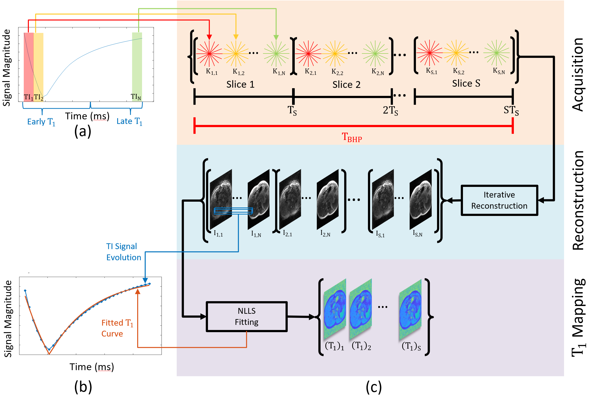
Figure 1: For
each slice, k-space data is acquired over a sampling period $$$T_{S}$$$. The total radial views for each slice are
split into $$$N$$$ TI groups
($$$K_{s,n} \quad s=1,...,S, \quad n=1,...,N$$$). The k-space data for each TI group are used
in an iterative reconstruction to obtain the TI images $$$I_{s,n}$$$. T1 maps for each slice are computed independently
at each spatial pixel by fitting an exponential model to the T1 recovery curve
using a nonlinear least squares method.
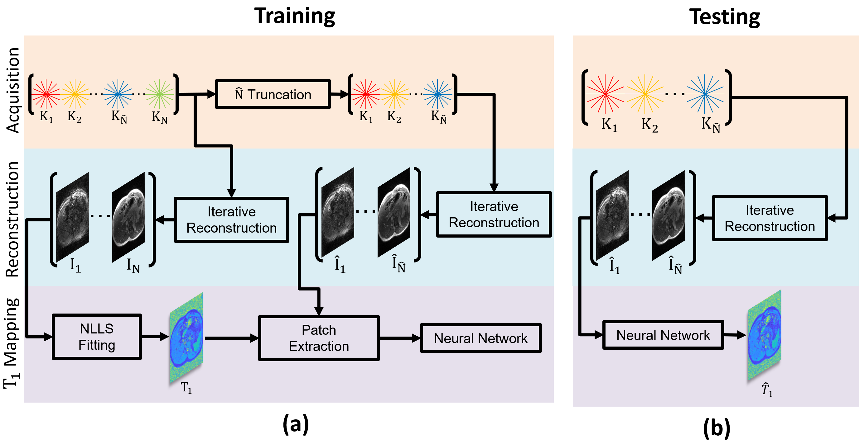
Figure 2: Demonstrating
the training (a) and testing (b) pipelines for deep learning based T1 mapping. In the figure, the pipelines are shown for a
single slice. During training, TI images are obtained with and without
truncation of the acquired k-space data along the T1 recovery curve (T1RC). The
images from the truncated T1RC k-space are used as input and the T1 map from
the full T1RC is used as target.
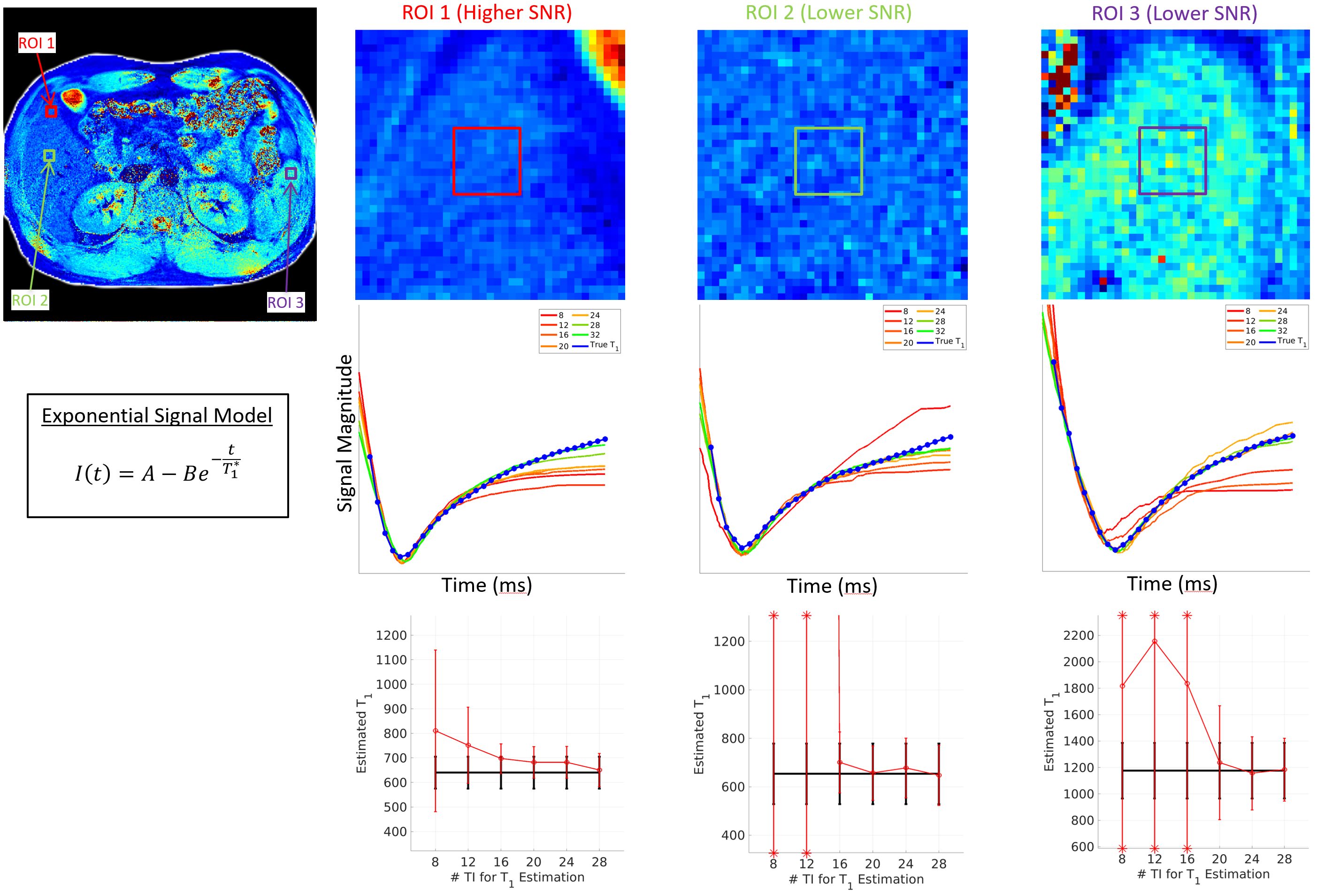
Figure 3: Demonstration
of T1 fitting performance using nonlinear least squares to fit the exponential
signal model. Row two provides the average fitted T1 curve for pixels within
each ROI, using varying amounts of TI data. The last row gives the average
estimated T1 value for pixels within each ROI, resulting from the corresponding
fitted curve in row two. Error bars represent the variation in T1 estimates
within each ROI, with * indicating values falling outside of the y-axis limits.
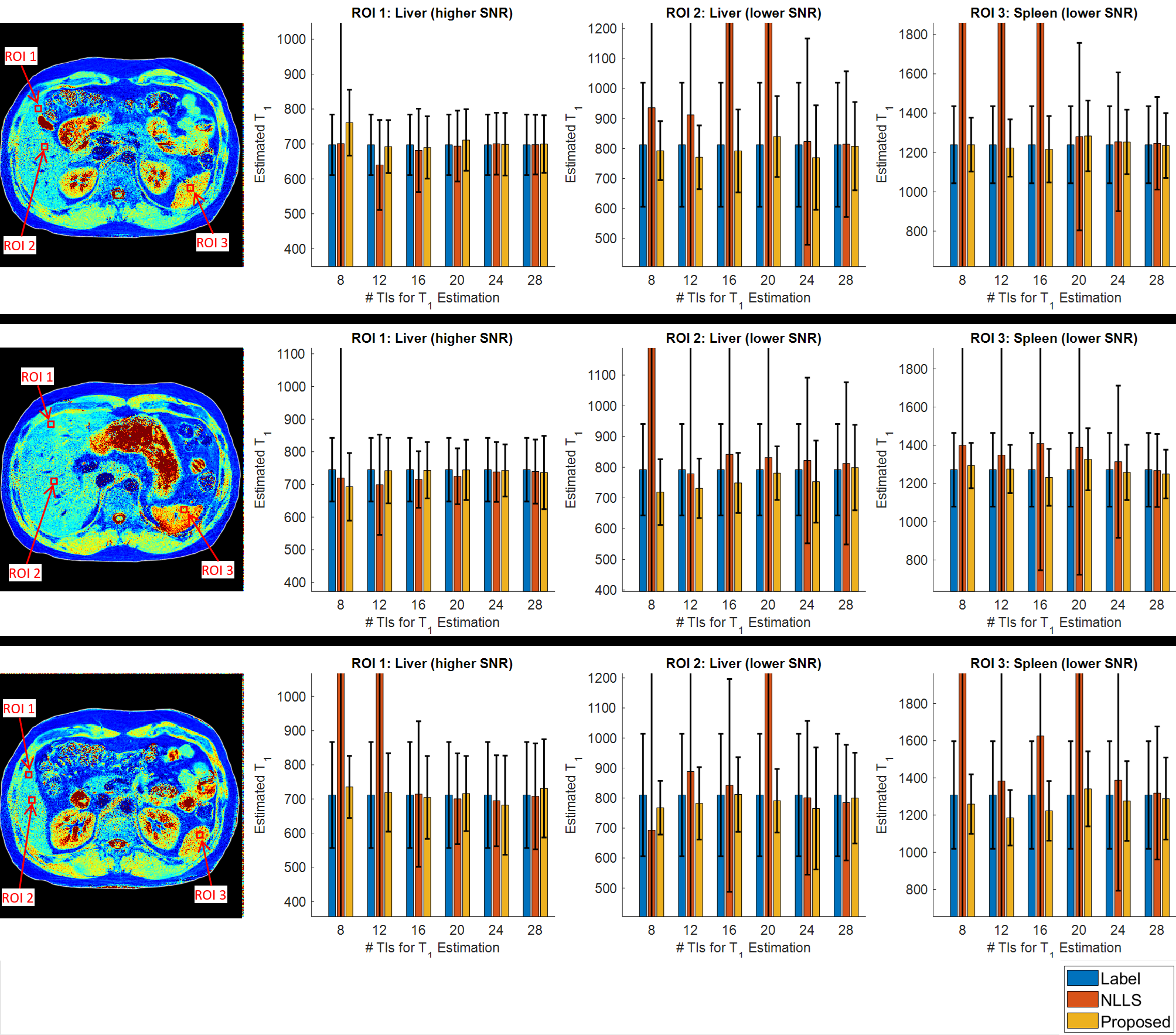
Figure 4: T1
estimation performance is shown for both the proposed DL framework and NLLS fitting
with $$$\hat{N}=8,12,16,20,24$$$ and $$$28$$$ TIs as
input. Results for three 9x9 pixel ROIs are given for three different slices.
The height of each bar represents the average T1 value within a given ROI, with
error bars representing the standard deviation.
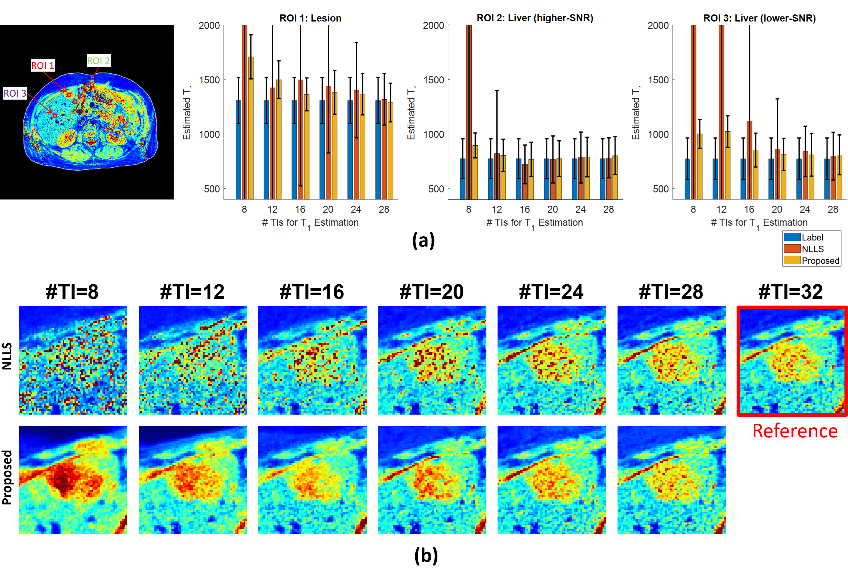
Figure 5: T1
estimation performance for a subject with a liver lesion for both the proposed DL
framework and NLLS fitting with $$$\hat{N}=8,12,16,20,24$$$ and $$$28$$$ and TIs as
input. In (a) results for three 9x9 pixel ROIs are given. The height of each
bar represents the average T1 value within a given ROI, with error bars
representing the standard deviation. In (b), visual examples are provided for
qualitative evaluation of the two techniques over the liver lesion with varying
TIs.