0600
Identifying Diffuse Intrinsic Pontine Glioma (DIPG) Subtypes via Radiomic Approaches
Silu Zhang1, Zoltan Patay1, Bogdan Mitrea2, Angela Edwards1, Lydia McColl Makepeace1, and Matthew A. Scoggins1
1Diagnostic Imaging, St. Jude Children's Research Hospital, Memphis, TN, United States, 2Activ Surgical, Boston, MA, United States
1Diagnostic Imaging, St. Jude Children's Research Hospital, Memphis, TN, United States, 2Activ Surgical, Boston, MA, United States
Synopsis
Diffuse intrinsic pontine glioma (DIPG) is a pediatric brain tumor with very poor prognosis. In this study, we identify two subtypes of DIPG based on radiomic features. The two subtypes show a significant difference in survival rates. Subtype 1 has a mean progression-free survival (PFS) and overall survival (OS) of 8.9 and 12.7 months, respectively. Subtype 2 has a mean PFS and OS of 5.7 and 9.1 months, respectively. Our results suggest that shape features and intensity features extracted from FLAIR and T1-post contrast predict the prognosis of DIPG.
INTRODUCTION
Diffuse intrinsic pontine glioma (DIPG) is a pediatric brain tumor with very poor prognosis. The median overall survival (OS) of patients is less than 1 year, and the 2-year survival rate is less than 10%.1 Studies have identified subgroups of DIPG based on genetic profiles.2-4 In this study, we identify DIPG subtypes based on radiomic features extracted from magnetic resonance imaging (MRI).METHODS
This study analyzed baseline imaging from 126 patients diagnosed with DIPG treated at St. Jude Children's Research Hospital. The workflow of image preprocessing and analysis is shown in Figure 1. For each patient, 4 MRI sequences were used for analysis: T1-weighted (T1-pre), T2-weighted (T2), T1-post contrast (T1-post), and T2 fluid-attenuated inversion recovery (FLAIR). All MRIs were co-registered, smoothed, bias corrected and intensity normalized using WhiteStripe5 normalization. Tumors were first auto segmented using Cascaded Anisotropic Convolutional Neural Networks6,7 and then manually adjusted by our image processing specialists if necessary. Radiomic features were extracted from segmented tumor regions using the PyRadiomics package.8 Original images and filtered images were used for calculating first order statistics, shape, and texture features. The bin width used for image discretization was customized for each image filter, such that the number of bins for each volume of interest was between 16 and 128 bins, as per PyRadiomics guidelines. This setup resulted in a total of 4746 features. Feature selection was then performed by measuring the dependence between the progression free survival (PFS) and each radiomic feature using distance correlation.9,10 Unlike Pearson correlation that measures only linear dependence (resulting in false negatives) and is sensitive to outliers (resulting in false positives), distance correlation measures the distance between 2 distributions and therefore ensures independence screening.11 Patients were randomly divided into training (80%) and validation (20%) sets, and feature selection was performed in only the training set. Features with P<0.05 were selected. Selected features were used for clustering analysis using unsupervised K-means clustering.12,13 The algorithm was first run on training data, and the centroid of each cluster was used to predict the cluster membership for validation data. To determine the best value for K, the K-means were run 100 times with random starting seeds on the training data for each value of K (2–4) and the K value resulting in the most stable cluster assignments was selected. The reproducibility of cluster assignment was measured by the average adjusted Rand index.14 After K was determined, the most frequent clustering assignment from the 100 runs was used for predicting validation data and survival analysis. The subtype determined by K-means clustering was then evaluated by survival prediction. Both PFS and OS were used as outcomes. Kaplan–Meier survival curves were plotted, and the Cox proportional hazard model was used to calculate the hazard ratio. The significance of difference in survival rates between different subtypes was tested by the log rank test.RESULTS
A total of 549 radiomic features with P<0.05 were selected. The K-means clustering analysis was first performed on the training set using the selected features, with K=2 providing the most reproducible results. For K=2, 3, and 4, the average adjusted Rand indexes were 0.97, 0.87, and 0.79, respectively. The partition results of K=2 on training and test data are shown in Figure 2. Frequencies of the 2 subtypes in our data are shown in Table 1, with the frequency of subtype 1 being 76% and subtype 2 being 24%. Survival rates of the 2 subtypes are shown in Figure 3. There was a significant difference in Kaplan–Meier curves of the 2 subtypes in both training data and validation data. For PFS, results showed P=0 on training and P=0.012 on validation. The hazard ratio (HR) between subtype 2 and subtype 1 was 2.48 for training and 3.53 for validation. Because of the high correlation between PFS and OS, subtypes assigned using PFS-related features could also accurately predict OS: P=0.006, HR=1.94 on training, and P=0.026, HR=3.05 on validation. The mean PFS and OS of the 2 subtypes are listed in Table 1. The mean PFS and OS of subtype 1 was 8.9 and 12.7 months and for subtype 2 was 5.7 and 9.1 months, respectively.DISCUSSION
Of 15 shape features extracted, 7 were selected. Of 542 intensity-based features selected, 268 were extracted from FLAIR, 168 from T1-post, 64 from T2, and 42 from T1. These results suggest that tumor shape, FLAIR, and T1-post intensity features (particularly nonuniformity, variance, energy, and contrast) inform the prognosis of DIPG.CONCLUSION
MRI imaging is the primary tool for diagnosis of DIPG. In one of the largest single institution cohorts of DIPG patients, radiomic features at baseline identified 2 subtypes with differing prognoses. Subtype 1 had a mean PFS and OS of 8.9 and 12.7 months, respectively. Subtype 2 had a mean PFS and OS of 5.7 and 9.1 months, respectively. A critical next step is to determine the relationship between these imaging-derived subtypes and genetic profiles. Biopsies have been historically performed infrequently due to the location of the tumor. The potential of subtyping by imaging information would be valuable.Acknowledgements
No acknowledgement found.References
- Hargrave, D., Bartels, U., & Bouffet, E. (2006). Diffuse brainstem glioma in children: critical review of clinical trials. The lancet oncology, 7(3), 241-248.
- Khuong-Quang, D. A., Buczkowicz, P., Rakopoulos, P., Liu, X. Y., Fontebasso, A. M., Bouffet, E., ... & Bourgey, M. (2012). K27M mutation in histone H3. 3 defines clinically and biologically distinct subgroups of pediatric diffuse intrinsic pontine gliomas. Acta neuropathologica, 124(3), 439-447.
- Buczkowicz, P., Hoeman, C., Rakopoulos, P., Pajovic, S., Letourneau, L., Dzamba, M., ... & Zuccaro, J. (2014). Genomic analysis of diffuse intrinsic pontine gliomas identifies three molecular subgroups and recurrent activating ACVR1 mutations. Nature genetics, 46(5), 451-456.
- Castel, D., Philippe, C., Calmon, R., Le Dret, L., Truffaux, N., Boddaert, N., ... & Mackay, A. (2015). Histone H3F3A and HIST1H3B K27M mutations define two subgroups of diffuse intrinsic pontine gliomas with different prognosis and phenotypes. Acta neuropathologica, 130(6), 815-827.
- Shinohara, R.T., et al., Statistical normalization techniques for magnetic resonance imaging. NeuroImage: Clinical, 2014. 6: p. 9-19.
- Wang, G., et al. Automatic brain tumor segmentation using cascaded anisotropic convolutional neural networks. in International MICCAI Brainlesion Workshop. 2017. Springer.
- Gibson, E., et al., NiftyNet: a deep-learning platform for medical imaging. Computer methods and programs in biomedicine, 2018. 158: p. 113-122.
- Van Griethuysen, J.J., et al., Computational radiomics system to decode the radiographic phenotype. Cancer research, 2017. 77(21): p. e104-e107.
- Székely, G.J. and M.L. Rizzo, Brownian distance covariance. The annals of applied statistics, 2009. 3(4): p. 1236-1265.
- Székely, G.J., M.L. Rizzo, and N.K. Bakirov, Measuring and testing dependence by correlation of distances. The annals of statistics, 2007. 35(6): p. 2769-2794.
- Li, R., W. Zhong, and L. Zhu, Feature screening via distance correlation learning. Journal of the American Statistical Association, 2012. 107(499): p. 1129-1139.
- Lloyd, S., Least squares quantization in PCM. IEEE transactions on information theory, 1982. 28(2): p. 129-137.
- MacQueen, J. Some methods for classification and analysis of multivariate observations. in Proceedings of the fifth Berkeley symposium on mathematical statistics and probability. 1967. Oakland, CA, USA.
- Hubert, L. and P. Arabie, Comparing partitions. Journal of classification, 1985. 2(1): p. 193-218.
Figures
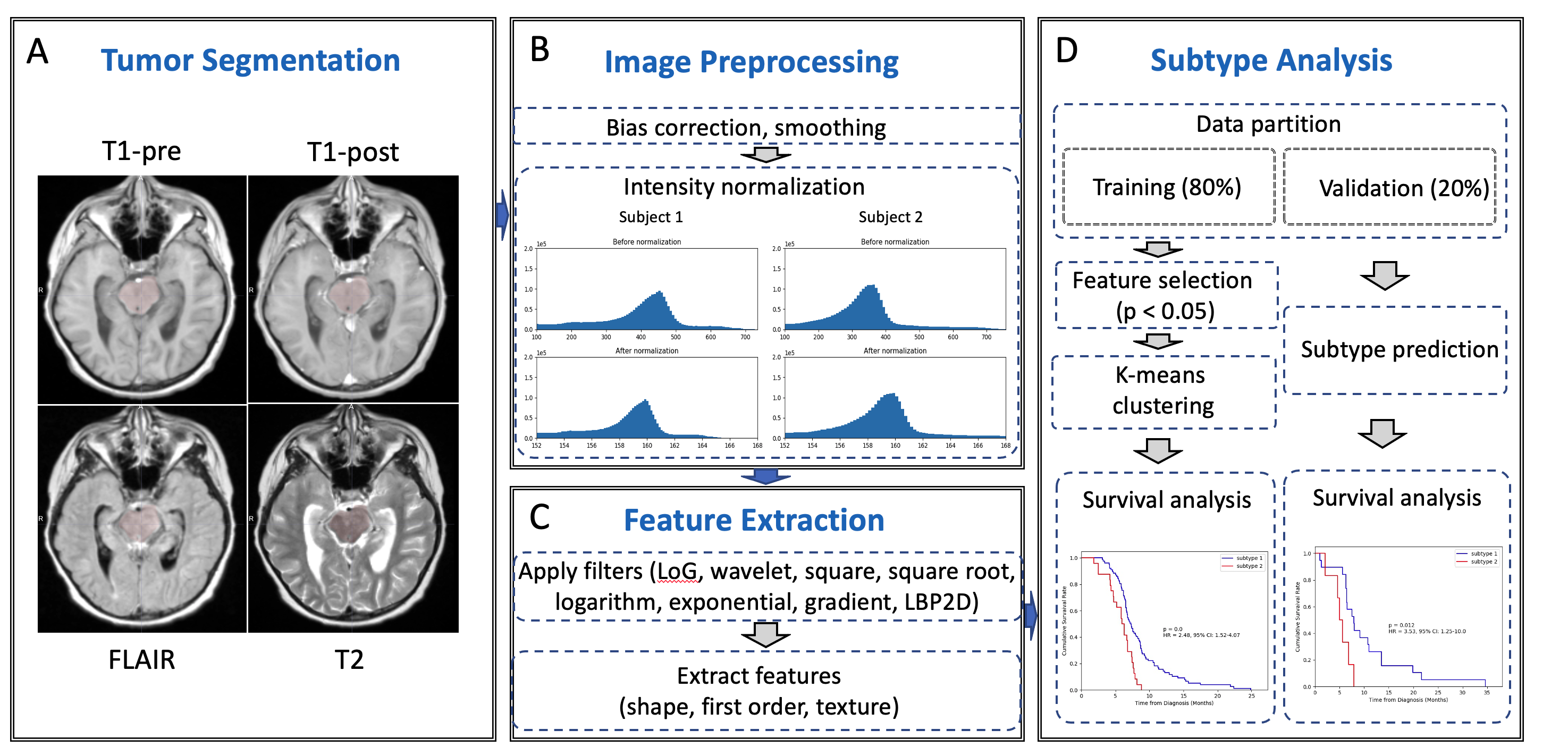
Figure 1.
Image preprocessing and analysis workflow. A) Images were first automatically
segmented and then manually adjusted if necessary. B) Images were bias
corrected, smoothed, and normalized. C) Radiomic features were extracted from
original and filtered images. D) Patients were divided into training (80%) and
validation (20%) sets. Feature selection was performed in only the training
set. Subtypes were identified using selected features, and survival analysis was
performed on the two subtypes identified.
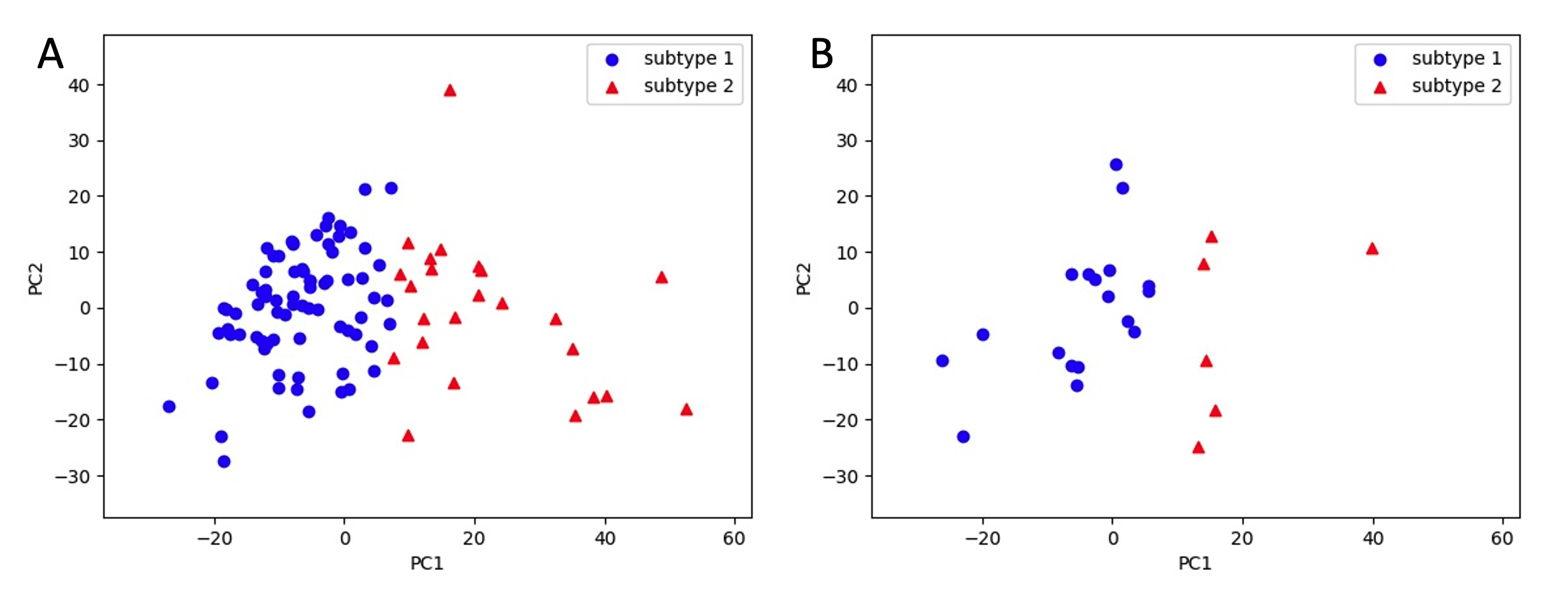
Figure 2. Identification
of two subtypes using selected features by K-means clustering. A) Training set.
B) Validation set.
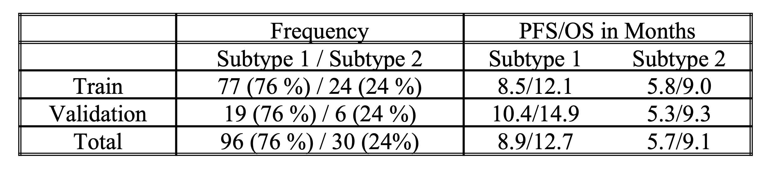
Table 1. Summary of frequency
and outcomes of the two subtypes identified in our study. PFS, progression free
survival; OS, overall survival.
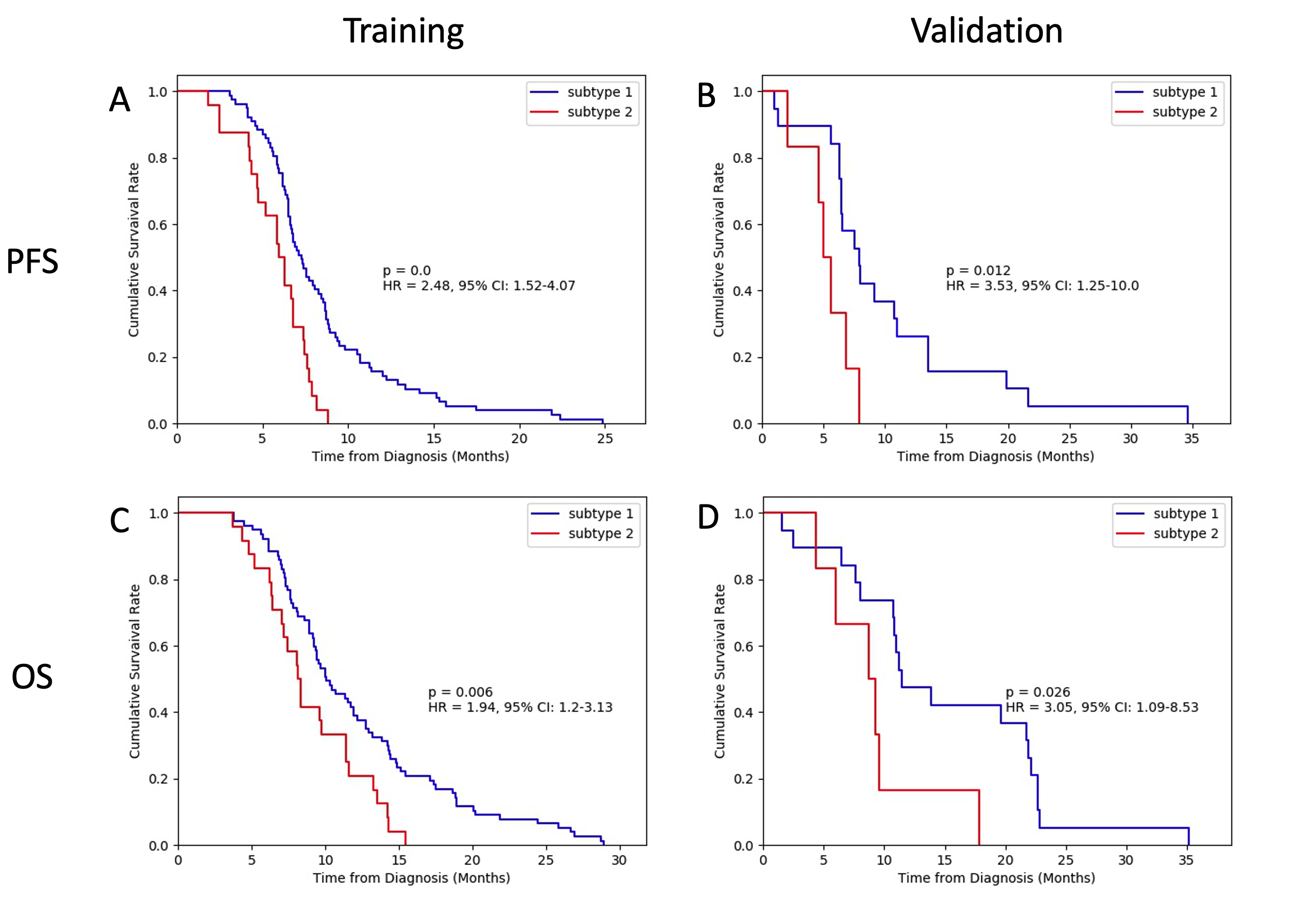
Figure 3.
Survival rates of the two subtypes identified. A) & B), progression free
survival (PFS). C) & D), overall survival (OS). A) & C) Training set.
B) & D) Validation set.