0587
The muscle twitch profile assessed with Motor Unit Magnetic Resonance Imaging (MUMRI)1Newcastle University Translational and Clinical Research Institute (NUTCRI), Newcastle University, Newcastle upon Tyne, United Kingdom, 2Newcastle Biomedical Research Centre, Newcastle University, Newcastle upon Tyne, United Kingdom, 3Northern Medical Physics and Clinical Engineering, Freeman Hospital, Newcastle upon Tyne NHS Foundation Trust, Newcastle upon Tyne, United Kingdom
Synopsis
Motor units (MUs) play a fundamental role in muscle physiology and disease. Contraction of muscle fibres belonging to a MU induces signal voids on diffusion weighted (DW) images enabling us to image these MUs (MUMRI). We demonstrated that MUMRI can also extract the twitch profile of single MUs. Computational modelling showed that the attenuation of net magnetisation and the cumulative phase changes increase with twitch magnitude. Therefore, we can measure the MU time profile by altering the timing of electrical nerve stimulation relative to the diffusion-encoding gradients. We applied this experimentally and measured in-vivo contraction times of human MUs.
Introduction
Each muscle has many motor units (MU) interdigitating across the muscle that allow control of muscle function.1 A MU comprises a lower motor neuron and the skeletal muscle fibres that this motor neuron innervates.1,2 When a motor neuron fires, the innervated muscle fibres contract, causing signal voids on diffusion weighted (DW) images allowing us to image activated MUs, a technique called MUMRI.3,4 MU activation can be controlled via electrical nerve stimulation, making it possible to activate a single MU.5 We hypothesized that by systematically shifting the electrical nerve stimulation timing in relation to the imaging acquisition window we can produce the twitch profile of this single MU.4 This would allow non-invasive discrimination of slow-twitch and fast-twitch MUs and assessment of how neuromuscular disorders alter the contractile properties of MUs. Adding to DW-MUMRI, a phase contrast (PC) sequence would enable quantification of velocity and displacement of contracting muscle fibres.6 Therefore, we investigated how different muscle twitch profiles affect the DW signal and PC signal using a computational model and by experimentally measuring twitch profiles of whole muscle and single MUs using DW and PC sequences.Computational modelling
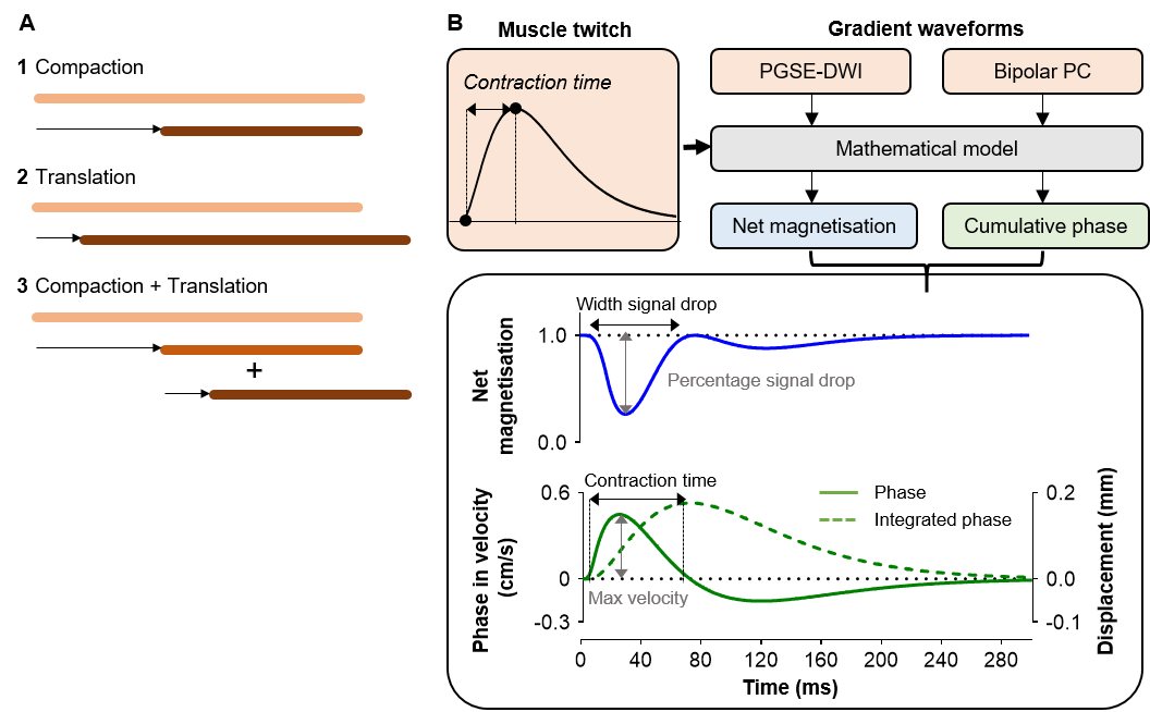
MethodsWe modelled the effect of a muscle contraction on a set of 1D points, representing elements of magnetisation. The displacement of each point was simulated as active contraction (compaction) or passive movement of adjacent inactive fibres (translation)(Fig.1A). Each model was applied in the presence of a PGSE DW imaging gradient (PGSE-DWI; b=20s/mm2, Δ/δ=16.9/2.2ms) and bipolar PC gradient (Bipolar-PC; VENC≈1.3cm/s, equal to b=5s/mm2, Δ/δ=9.13/4.57ms)(Fig.1B). These gradient waveforms were stepped in time across a twitch waveform to simulate the effect of moving the nerve stimulus in time relative to the encoding gradients on the DW and PC signal. For each step, we calculated the magnitude of the net magnetisation and cumulative phase (Fig.1B)
Results
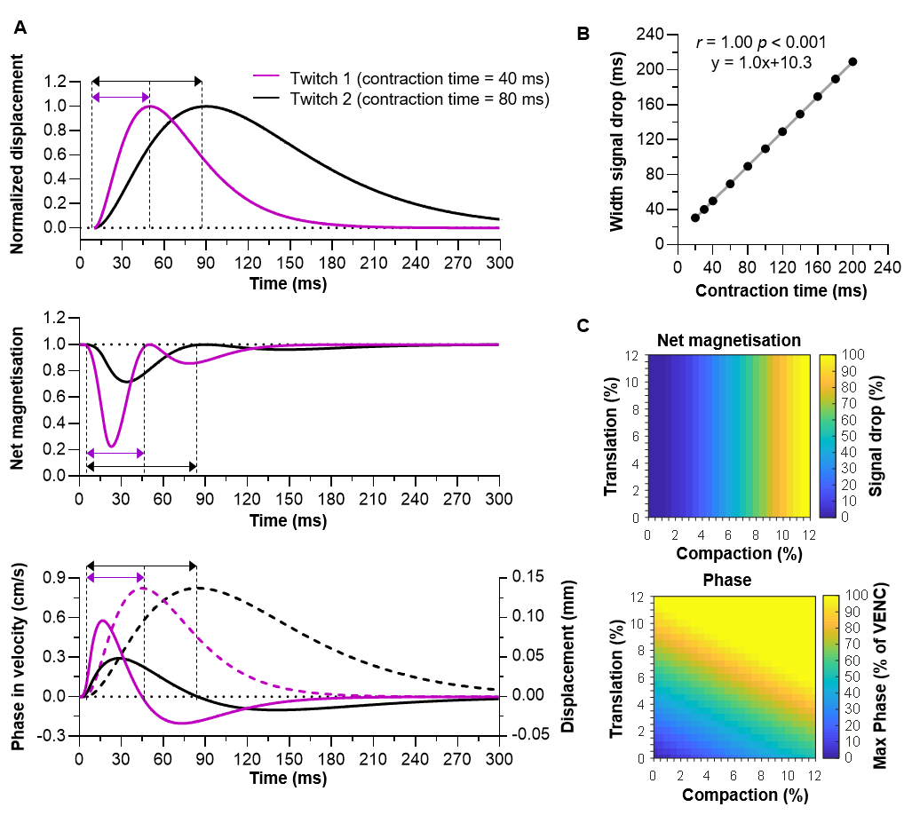
During compaction, the net magnetisation modelled with PGSE-DWI exhibited two consecutive drops, while the cumulative phase modelled with Bipolar-PC showed a positive peak followed by a negative peak (Fig.2A). These two phases coincide with the contraction and relaxation in the muscle twitch. The theoretical twitch contraction time was linearly related to the width of the first signal drop in net magnetisation and PC contraction time (both r=1.00, p<0.001; Fig.2B). The drop in net magnetisation increased with more compaction, while the maximum velocity measured with Bipolar-PC was increased with more compaction and more translation (Fig.2C).
Experimental measurements
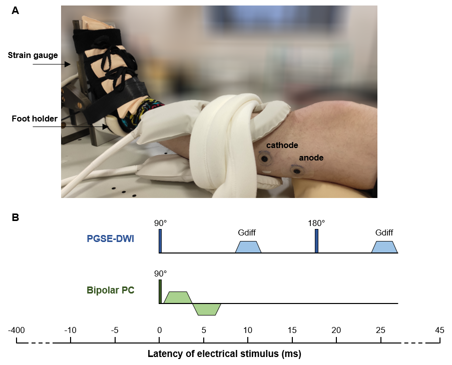
MethodsDesign: We scanned the left lower leg of 10 healthy volunteers with a 3T Philips MR scanner using a flexM coil (Fig.3A). The peroneal or tibial nerve was electrically stimulated at a current producing a visible muscle twitch (Imuscle) and at a current activating a single MU (IsingleMU).
Data-acquisition: For Imuscle and IsingleMU, the muscle twitch was assessed by acquiring 90 axial DW images (1/sec; FOV=160x160mm, resolution=1.5x1.5x7.5-8mm, TR/TE=1000/36-37ms, Δ/δ=16.9/2.2ms, b=20s/mm2, sensitization=feet-head, fat suppression=SSGR+SPAIR). For each image, the timing between the stimulus and 90° RF pulse was changed (step=5ms, from +50ms to -400ms; Fig.3B), thereby stepping the PGSE-DWI across the muscle twitch profile. At IsingleMU, this process was repeated for the PC sequence (TR/TE=500-700/9.7-15.2ms, VENC=1-5cm/s). At Imuscle, the force twitch was measured with an MR compatible force transducer (Fig.3A).
Data-processing: The stimulated muscle or single MU was delineated on the DW scan and the average signal intensity was determined per latency step to create a latency DW profile. For IsingleMU, the velocity profile was extracted from the PC images and integrated to a displacement profile. We determined the contraction time from the force twitch and PC displacement profile and the width of the first signal drop from the DW latency profile.
Results
Imuscle: The DW latency profile at Imuscle (13.4±6.1mA) showed two consecutive signal drops, reflecting the contraction and relaxation of the muscle (Fig.4A/B). The width of the first signal drop (mean±SD: 103±20ms) was comparable to the force contraction time (93±34ms; intra-class correlation (ICC)=0.717, p=0.010; fig.4C).
IsingleMU: During the contraction, the stimulated MU (IsingleMU=8.6±3.3mA) became black on the DW images and showed a positive velocity on the phase images (0.55±0.26cm/s) followed by a negative velocity (-0.22±0.10cm/s) during relaxation (Fig.5A/B). Voxel-wise analysis revealed localized DW changes occurring together with wide-spread phase changes (Fig.5C).
Discussion and conclusion
We demonstrated that compaction is the primary contrast mechanism for observed signal voids in DW images of active muscle, meaning that DW-MUMRI only detects the MU’s active part. Phase changes were more wide-spread reflecting neighbouring fibres that are passively pulled along (translation). The amplitude of the DW signal attenuations and phase changes increased with twitch magnitude enabling us to measure MU twitch profiles by altering the timing of stimulation in relation to the imaging acquisition window. Doing so, we measured contraction times of single MUs with DW-MUMRI and PC-MUMRI, which were close to values reported in literature for lower leg MUs (40-110ms).7,8 In conclusion, MUMRI can measure the time dynamics and contractile velocity of single MUs, all in a clinically feasible 30 minute scan time. Therefore, MUMRI would offer a way to study the preferential loss of fast-twitch MUs and the resulting transition of fast-twitch muscle fibres to slow-twitch muscle fibres that occurs in neuromuscular disorders.9,10Acknowledgements
Acknowledgements: We like to thank Dr. Kieren Hollingsworth for his help developing a software patch for the Philips 3T Achieva system which enabled the use of a phase contrast sequence with an echo planar read out scheme. Furthermore, we like to thank Sean Johnson and the radiographers for their help with the data-acquisition.
Funding: This work was supported by the Rubicon research programme (project number: 452183002) of the Dutch Research Council (NWO), by the Medical Research Council Confidence in Concept (CiC) award [Newcastle University study number 1621/7484/2018], by Muscular Dystrophy UK [grant number: 18GROPG36-0246-1] and the NIHR Newcastle Biomedical Research Centre. The NIHR Newcastle Biomedical Research Centre (BRC) is a partnership between Newcastle Hospitals NHS Foundation Trust and Newcastle University, funded by the National Institute for Health Research (NIHR). This paper presents independent research funded and supported by the NIHR Newcastle BRC. The views expressed are those of the author(s) and not necessarily those of the NIHR or the Department of Health and Social Care.
References
1. Buchthal F, Schmalbruch H. Motor unit of mammalian muscle. Physiol Rev. 1980;60(1):90-142. doi:10.1152/physrev.1980.60.1.90
2. Heckman CJ, Enoka RM. Motor Unit. In: Comprehensive Physiology. Vol 2. ; 2012:2629-2682. doi:10.1002/cphy.c100087
3. Steidle G, Schick F. Addressing spontaneous signal voids in repetitive single-shot DWI of musculature: Spatial and temporal patterns in the calves of healthy volunteers and consideration of unintended muscle activities as underlying mechanism. NMR Biomed. 2015;28(7):801-810. doi:10.1002/nbm.3311
4. Whittaker RG, Porcari P, Braz L, Williams TL, Schofield IS, Blamire AM. Functional magnetic resonance imaging of human motor unit fasciculation in amyotrophic lateral sclerosis. Ann Neurol. 2019;85(3):455-459. doi:10.1002/ana.25422
5. Birkbeck MG, Heskamp L, Schofield IS, Blamire AM, Whittaker RG. Non-invasive imaging of single human motor units. Clin Neurophysiol. 2020;131(6):1399-1406. doi:10.1016/j.clinph.2020.02.004
6. Pelc NJ, Herfkens RJ, Shimakawa A, Enzmann DR. Phase contrast cine magnetic resonance imaging. Magn Reson Q. 1991;7(4):229-254.
7. Leitch M, Macefield VG. Comparison of contractile responses of single human motor units in the toe extensors during unloaded and loaded isotonic and isometric conditions. J Neurophysiol. 2015;114(2):1083-1089. doi:10.1152/jn.00121.2015
8. Andreassen S, Arendt-Nielsen L. Muscle fibre conduction velocity in motor units of the human anterior tibial muscle: a new size principle parameter. J Physiol. 1987;391(1):561-571. doi:10.1113/jphysiol.1987.sp016756
9. Hegedus J, Putman CT, Tyreman N, Gordon T. Preferential motor unit loss in the SOD1 G93A transgenic mouse model of amyotrophic lateral sclerosis. J Physiol. 2008. doi:10.1113/jphysiol.2007.149286
10. Frey D, Schneider C, Xu L, Borg J, Spooren W, Caroni P. Early and selective loss of neuromuscular synapse subtypes with low sprouting competence in motoneuron diseases. J Neurosci. 2000;20(7):2534-2542. doi:10.1523/JNEUROSCI.20-07-02534.2000
Figures