0567
Head Motion Tracking using an EEG-system and Retrospective Correction of High-Resolution T1-weighted MRI1Section for Magnetic Resonance, DTU Health Tech, Technical University of Denmark, Kgs. Lyngby, Denmark, 2Danish Research Centre for Magnetic Resonance, Centre for Functional and Diagnostic Imaging and Research, Copenhagen University Hospital Hvidovre, Hvidovre, Denmark, 3Sino-Danish Center, University of Chinese Academy of Sciences, Beijing, China, 4Philips Healthcare, Copenhagen, Denmark, 5State Key Laboratory of Brain and Cognitive Science, Beijing MR Center for Brain Research, Institute of Biophysics, Chinese Academy of Sciences, Beijing, China, 6Beijing Institute for Brain Disorders, Beijing, China, 7DTU Compute, Technical University of Denmark, Kgs. Lyngby, Denmark
Synopsis
Tracking and retrospective correction of high-resolution structural 3D-GRE images is accomplished with a slightly modified EEG cap and sampling system. Carbon wire loops added to the EEG cap allow for motion tracking using gradient-induced signals from native sequence elements, without the need for sequence modification, or electrode-skin contact, while requiring only a short calibration scan, and mounting of the cap. The motion estimates closely resemble estimates from interleaved navigators (mean absolute difference: [0.13,0.33,0.12]mm, [0.28,0.15,0.22]deg). Retrospective correction using carbon wire loops yield similar improvements to Average Edge Strength (12%) for images with instructed movement, and does not degrade images without motion.
Introduction
Sensors consisting of orthogonally arranged gradient pickup-coils fixed to the subjects head have proven useful for motion tracking when combined with interleaved gradients or tones.1,2 Pilot studies have shown that tracking is possible during simultaneous EEG-fMRI using only EEG-equipment sensitive to field changes.3-8 With a modified EEG setup including carbon wire loops, and after a short calibration scan, motion tracking is achieved using native gradients of a high-resolution T1w 3D-GRE sequence, requiring only a short calibration scan and mounting of the cap. The method is validated with retrospective correction for three healthy subjects, with direct comparison to interleaved 3D navigators (NAVs)9.Methods
Gradient switching induces voltages in the wire loops and it follows from Faraday's law that the recorded time signal of channel $$$i$$$ can be described as: $$\mathit{v}_i(t)=\mathit{w}_{ix}\frac{\partial\tilde{\mathit{g}}_x(t)}{\partial t}+\mathit{w}_{iy}\frac{\partial\tilde{\mathit{g}}_y(t)}{\partial t}+\mathit{w}_{iz}\frac{\partial \tilde{\mathit{g}}_z(t)}{\partial t}+\mathit{\eta}_i(t)$$with $$$\dot{\tilde{\pmb{\mathit{G}}}}(t)=\left[\frac{\partial \tilde{\mathit{g}}_x(t)}{\partial t},\frac{\partial\tilde{\mathit{g}}_y(t)}{\partial t},\frac{\partial \tilde{\mathit{g}}_z(t)}{\partial t}\right]$$$ representing filtered time derivatives of gradient activity, and $$$\pmb{\mathit{w}}_i=\left[\mathit{w}_{ix},\mathit{w}_{iy},\mathit{w}_{iz}\right]$$$ being weights that depend on wire loop geometry, position, and orientation. $$$\mathit{\eta }_i(t)$$$ is measurement noise. $$$\dot{\tilde{\pmb{\mathit{G}}}}(t)$$$ is recorded for any sequence, for each of the gradients $$$\mathit{g}_x(t)$$$, $$$\mathit{g}_y(t)$$$, and $$$\mathit{g}_z(t)$$$, in a static phantom pre-scan (Figure 1) where RF and the remaining gradient systems are deactivated, and is determined as the primary component from singular value decomposition (SVD) across wire loop channels $$$i=[1,2,\ldots ,I]$$$. $$$\pmb{\mathit{w}}_i$$$ is determined for a new signal snippet using a general linear model expressed by $$$\dot{\tilde{\pmb{\mathit{G}}}}(t)$$$. Additional nuisance regressors are appended to $$$\dot{\tilde{\pmb{\mathit{G}}}}(t)$$$ to model $$$\mathit{\eta }_i(t)$$$. These are determined in the pre-scan by sampling RF contributions without gradients (Figure 1,RF), and by modelling eddy currents and cross talk by including non-primary components from the aforementioned SVD. Additionally, mechanical vibrations are modelled with a low-frequency harmonic expansion [120-400Hz] fitted to periods free of gradient ramping (Figure 2), and are subtracted.
The relation between weights $$$\pmb{\mathit{w}}$$$ ($$$3I$$$ vector) and subject pose $$$\pmb{\mathit{r}}$$$ (position and orientation, six degrees-of-freedom), is determined in a short subject-specific calibration scan with instructed free head movement during a dynamic series of rapid 3D-EPI. Small changes in subject pose from a reference position corresponds to small changes in $$$\pmb{\mathit{w}}$$$ in the linear approximation:
$$\Delta\pmb{\mathit{w}}=\pmb{\mathit{A}}\Delta\pmb{\mathit{r}}$$
where $$$\Delta\pmb{\mathit{w}}=\left[\Delta\pmb{\mathit{w}}_{1},\Delta\pmb{\mathit{w}}_{2},\ldots ,\Delta\pmb{\mathit{w}}_{I}\right]$$$, and $$$\Delta\pmb{\mathit{r}}=\left[\Delta x,\Delta y,\Delta z,\Delta \theta ,\Delta \phi,\Delta \psi \right]$$$. The elements of $$$\pmb{\mathit{A}}$$$ ($$$3I\times 6$$$ matrix) are found by jointly solving the linear approximation for a number ($$$\geq 6$$$) of calibration positions by least squares estimation, using motion parameters from rigid alignment of the 3D-EPI volumes (SPM12 volume realignment, UCL, UK).
The developed method was evaluated in-vivo using three healthy volunteers. An 80s calibration scan, and four structural T1w 3D-GRE images (all with NAVs), were acquired for each subject (3T Achieva MRI, Philips Healthcare, Best, Netherlands). Subjects were instructed to remain stationary during 2 structural scans, and to perform various amounts of voluntary motion for 2 scans. The structural scans were retrospectively corrected using the RetroMoCoBox10 with pose estimates from either rigid alignment (SPM12) of NAVs9 (recorded every 1561ms interleaved11,12 with acquiring slices of k-space), or from carbon wire loop (CWL) recordings. Loop recordings during interleaved navigators were excluded from pose estimation for fair comparison between the two methods. The sequence used during calibration was identical to the interleaved NAVs with sequence parameters TE/TR: 5.8/14ms, duration per dynamic: 472ms, tip angle: 2°, voxel size: 7.1×8.2×7.2mm, matrix: 36×31×32. Sequence parameters for the T1w 3D-GRE images were TE/TR: 3.5/6.5ms, tip angle: 14°, voxel size: 1×1×1mm, matrix: 240×240×240, outer/inner phase-encoding order: center-out/linear.
CWL voltages were sampled with a high bandwidth EEG sampling system (80kHz sampling, HP/LP-cutoffs: 100Hz/16kHz, NeurOne Tesla, Bittium Biosignals Ltd, Kuopio, Finland), and an EEG-cap (Easycap, Germany) with 9 channels interconnected to the reference electrode with resistive carbon wire forming inductive loops evaluated for safety. CWL motion estimation was based on signals from two consecutive dynamics with 50% overlap yielding 1561ms tracking frequency.
Average Edge Strength (AES) was calculated before and after retrospective correction using the AES toolbox13, averaging over sagittal, coronal, and axial orientation. Before calculation, reference, corrupted, and corrected images were transformed to a common reference frame using sinc interpolation.
Results
Figure 3 and 4 show retrospectively corrected volumes with instructed-, and uninstructed movement respectively. Table 1 shows AES for each structural scan, before and after retrospective correction. The average improvement to AES in volumes with instructed movement was 12/13% for CWL and NAVs, respectively, and -0.39/1.8% in volumes where the subject was instructed to lay still. The average mean absolute difference (MAD) for all structural scans between CWL pose estimates and NAVs estimates were [0.13,0.33,0.12]mm and [0.28,0.15,0.22]deg, revealing close similarity between the two.Discussion & Conclusion
While comparable in terms of improvements to image sharpness (visually and calculated AES), CWLs can offer decreased tracking noise, especially in anterior/posterior direction, where NAVs are most sensitive to field fluctuations. Neither method introduced noise in motion-free scans. No line-of-sight or sequence modification was needed for CWL. The method is suited for prospective updating, which requires scanner interfacing and updating of three columns of $$$\dot{\tilde{\pmb{\mathit{G}}}}(t)$$$ whenever the field-of-view is updated5. Residual artifacts from local Nyquist violations in k-space may improve with prospective updating, and reacquisition. CWLs for EEG artifact rejection have recently become commercially available, and may be suited for the method.Acknowledgements
Malte Laustsen is supported by the Sino-Danish Center for Education and Research.References
[1]. Roth A, Nevo E. Method and apparatus to estimate location and orientation of objects during MRI. US patent 2010028. 2010.
[2]. van Niekerk A, van der Kouwe A, Meintjes E. Toward “plug and play” prospective motion correction for MRI by combining observations of the time varying gradient and static vector fields. Magn Reson Med 2019;82:1214–1228 doi: 10.1002/mrm.27790.
[3]. Vestergaard MB, Schulz J, Turner R, Hanson LG. Motion tracking from gradient induced signals in electrode recordings. In: ESMRMB Congress, 2011.
[4]. Wong C-K, Zotev V, Misaki M, Phillips R, Luo Q, Bodurka J. Automatic EEG-assisted retrospective motion correction for fMRI (aE-REMCOR). NeuroImage 2016;129:133–147 doi: 10.1016/j.neuroimage.2016.01.042.
[5]. Andersen M, Madsen KH, Hanson LG. Prospective motion correction for MRI using EEG-equipment. In: ISMRM 24th Conference, Singapore; 2016.
[6]. Bhuiyan EH, Spencer G, Glover PM, Bowtell R. Tracking head movement inside an MR scanner using voltages induced in coils by time-varying gradients. In: ISMRM 25th Conference, Honolulu, United States; 2017.
[7]. Laustsen M, Andersen M, Madsen KH, Hanson LG. Gradient distortions in EEG provide motion tracking during simultaneous EEG-fMRI. In: ISMRM Workshop on: Motion Correction in MRI & MRS, Cape Town, South Africa; 2017.
[8]. Laustsen M, Andersen M, Lehmann PM, Xue R, Madsen KH, Hanson LG. Slice-wise motion tracking during simultaneous EEG-fMRI. In: ISMRM 26th Conference, Paris, France; 2018.
[9]. Tisdall MD, Hess AT, Reuter M, Meintjes EM, Fischl B, van der Kouwe AJW. Volumetric Navigators (vNavs) for Prospective Motion Correction and Selective Reacquisition in Neuroanatomical MRI. Magn Reson Med 2012;68:389–399 doi: 10.1002/mrm.23228.
[10]. Gallichan D, Marques JP, Gruetter R. Retrospective correction of involuntary microscopic head movement using highly accelerated fat image navigators (3D FatNavs) at 7T. Magnetic Resonance in Medicine 2016;75:1030–1039 doi: 10.1002/mrm.25670.
[11]. Henningsson M, Mens G, Koken P, Smink J, Botnar RM. A new framework for interleaved scanning in cardiovascular MR: Application to image-based respiratory motion correction in coronary MR angiography. Magnetic Resonance in Medicine 2015;73:692–696 doi: https://doi.org/10.1002/mrm.25149.
[12]. Andersen M, Björkman-Burtscher IM, Marsman A, Petersen ET, Boer VO. Improvement in diagnostic quality of structural and angiographic MRI of the brain using motion correction with interleaved, volumetric navigators. PLOS ONE 2019;14:e0217145 doi: 10.1371/journal.pone.0217145.
[13]. Zacà D, Hasson U, Minati L, Jovicich J. Method for retrospective estimation of natural head movement during structural MRI. Journal of Magnetic Resonance Imaging 2018;48:927–937 doi: 10.1002/jmri.25959.
Figures
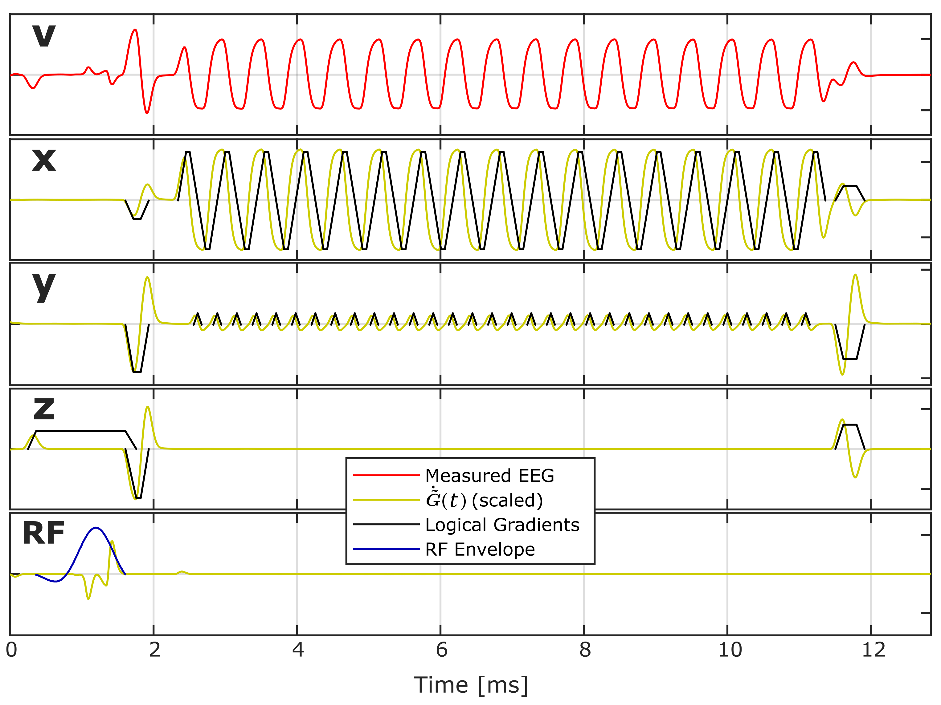
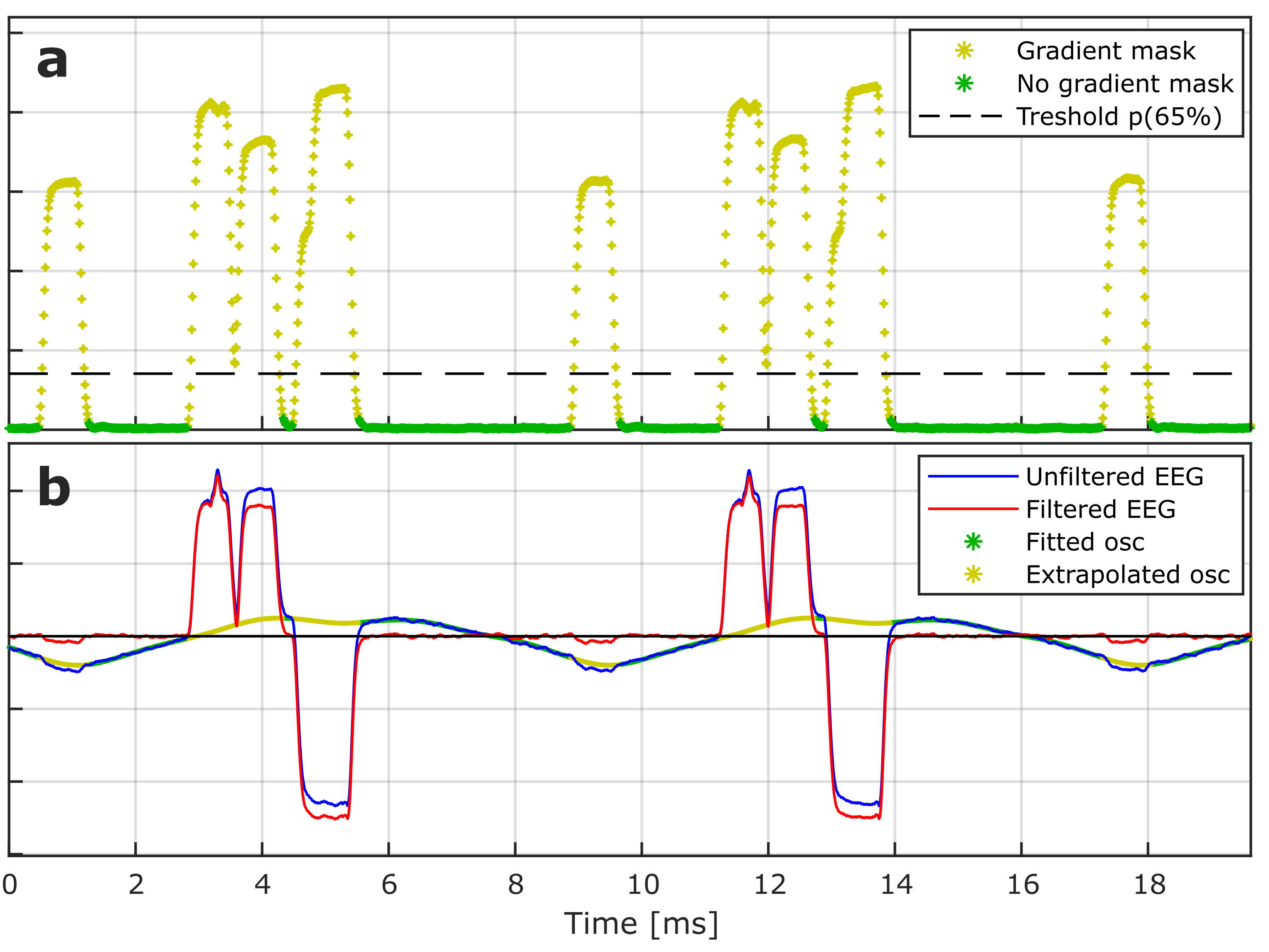
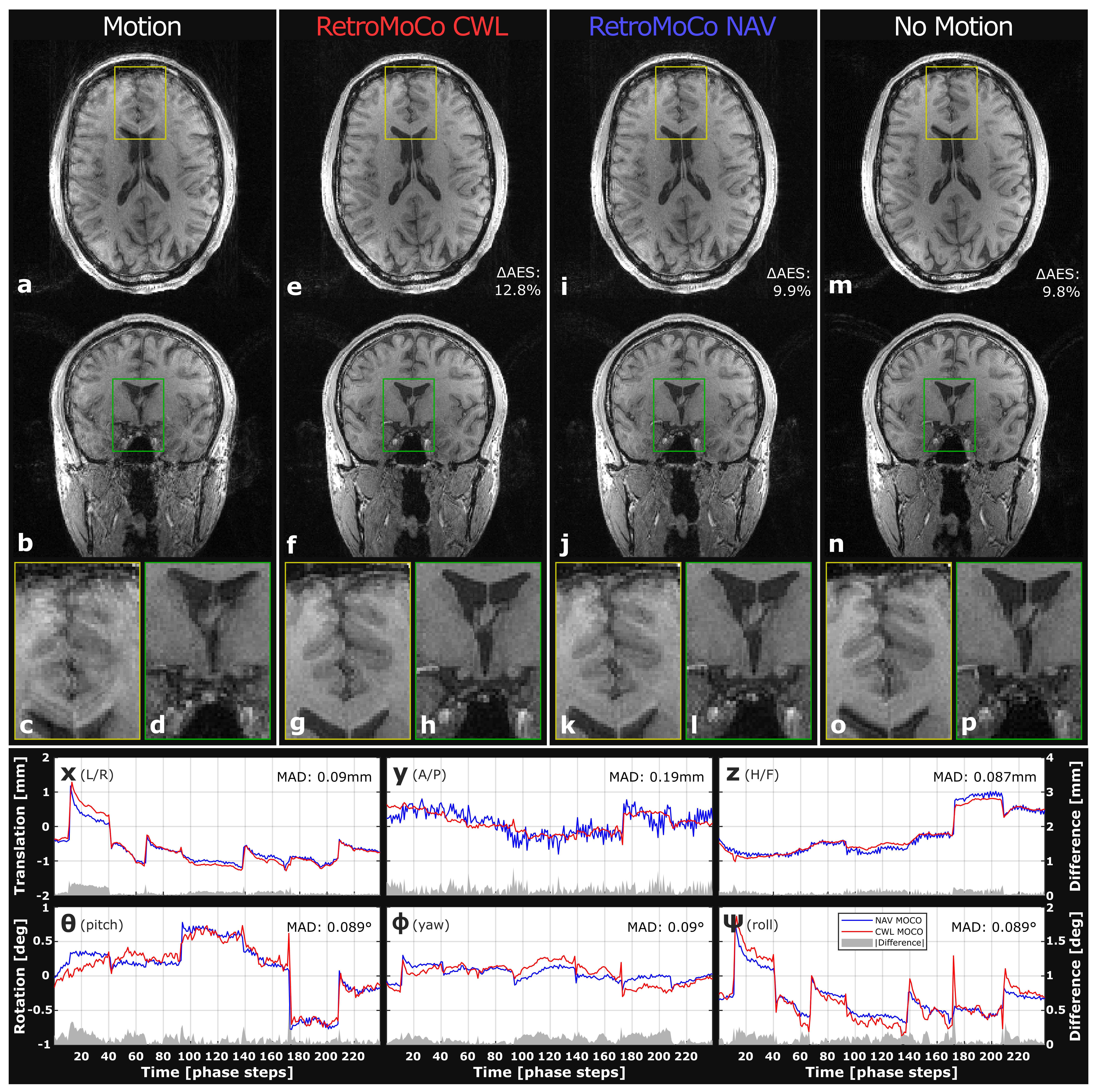
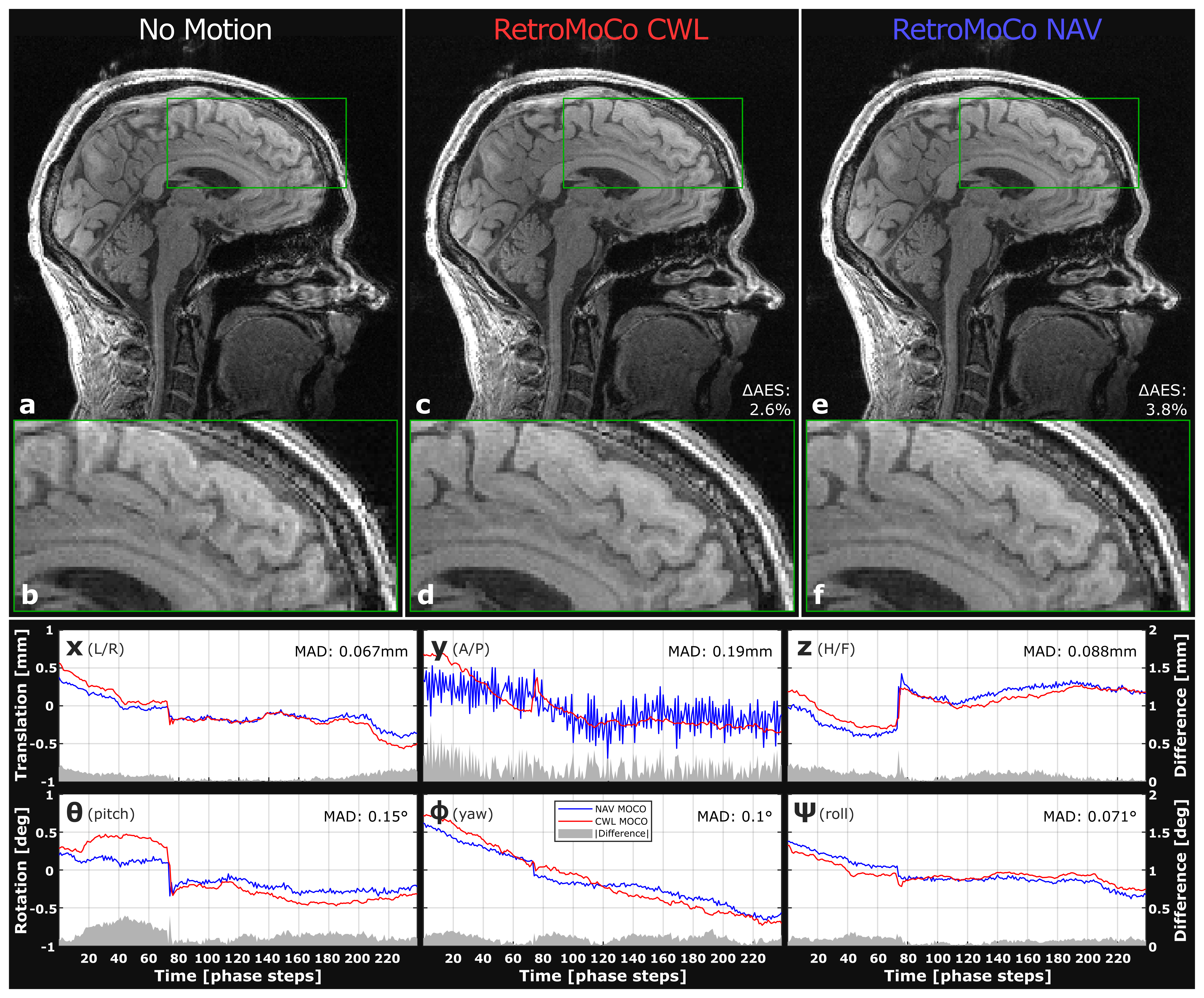

Table1: Average Edge Strength (AES) before and after retrospective correction of every high-resolution structural 3D-GRE scan. All absolute AES values are scaled by 10^5 for convenient displaying. Average improvement to AES: 12/13% for CWL/NAV in instructed movement (trials 3, and 4), and -0.39/1,8% for CWL/NAV while laying still (trials 1, and 2).