0557
Fast T1 mapping and weighting MRI in preclinical and clinical settings using subspace-constrained joint-domains reconstructions1Department of Chemical and Biological Physics, Weizmann Institute of Science, Rehovot, Israel, 2Department of Electronic Science, Xiamen University, Xiamen, China
Synopsis
Fast T1 mapping methods based on subspace-constrained reconstructions of jointly sparsed-sample domains, are proposed and shown to efficiently deliver maps with either multiple T1 contrasts or T1 values with ≈ 50-100× accelerations. Both single-shot and multi-shot implementations were developed, incorporating random-sampling inversion recovery (IR) as well as variable-TR multi-shot gradient echo (GRE) and spatiotemporally encoded (SPEN) sequences. In vivo human brain scans confirmed the efficiency of this method. Preclinical scans on kidneys and on tumor-implanted animals subject to dynamic contrast-enhanced T1 mapping, also demonstrate the proposed method's advantages for functional and pathological diagnoses.
Introduction
Recent years have seen significant advances in schemes for accelerating parametric imaging, based on subspace-constrained (SC) sampling.1-5 By speeding up acquisitions, this can overcome motions and probe dynamic effects. The present work uses SC techniques to deliver images at multiple T1 contrast and T1 maps in a seconds timescale. Random-sampling inversion recovery (IR) gradient echo (GRE) and variable TR (VTR) Spatiotemporal Encoding (SPEN) methods,6-9 were tested in these acquisitions. The accuracy of the proposed methods was compared against more conventional, longer acquisitions, in both clinical and preclinical scanners. Improved clinical (brain) and preclinical scans on kidneys and on tumor-implanted animals subject to dynamic-contrast-enhanced T1 mapping demonstrate the method's advantages for functional and pathological diagnoses.Methods
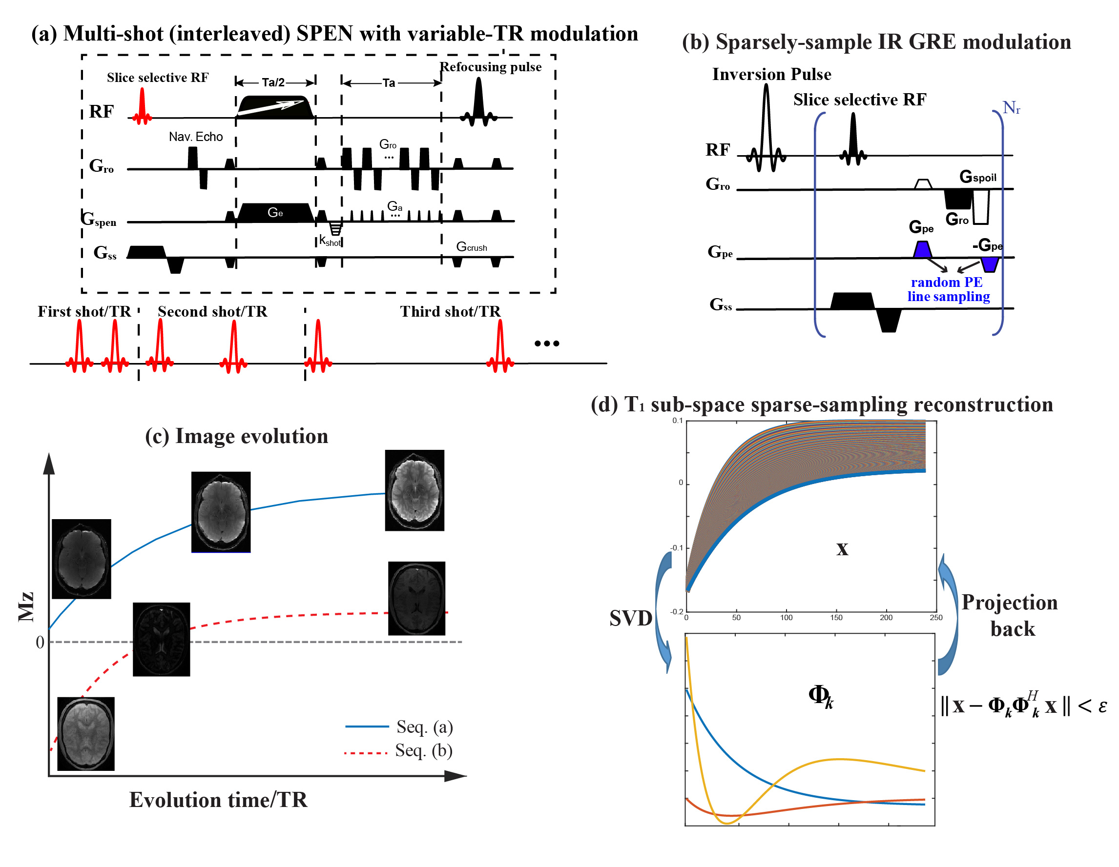
Theoretical background. Figure 1a shows one of the schemes assayed, involving a VTR acquisition in conjunction with interleaved SPEN. For each TR a single SPEN shot was acquired; VTR is then combined with interleaving to obtain the final data. Figure 1b shows an alternative based on the IR GRE sequence, starting with an inversion pulse and followed by small-tip-angle GRE readouts that are sparsely encoded both in phase and in their IR times. Figure 1c describes the image evolution of the two sequences, which share partial image sampling in conjunction with different T1 weightings. Figure 1d presents the scheme taken for the SC joint-domain reconstruction. In this scheme $$$\bf x$$$ represents the matrix being sought, of all the full-resolution images along with their T1 weights. Calling y the data matrix collected, the reconstruction is performed by solving the minimization problem:$$ \min_{\omega}\frac{1}{2}\parallel{\bf y}-{\bf E}{\bf \Phi}_{k}\omega\parallel_2^2+\lambda\sum_r\parallel{\bf R\scriptsize r}\left(\omega\right)\parallel\scriptsize*$$ (1)
Here $$$ \omega={\bf \Phi}_k^H\bf x $$$ is an array of subspace coefficient summarizing the T1 dependence of the images, after the subspace of all realistic $$${\bf \Phi}_{\it k}$$$ signal evolutions are calculated and expanded into a minimal component basis satisfying$$$\parallel {\bf x}-{\bf \Phi}_{\it k}{\bf \Phi}_{\it k}^Hx\parallel$$$(Figure 1d). 2,10
Data acquisition. Human volunteers were scanned following IRB approvals by the Wolfson Medical Center (Israel) and the Weizmann Institute, and collected after informed consent on a 3T Prisma Siemens MRI using a 32-channel head coil. Reference T1 maps were collected using the TGSE sequence in the Siemens' library; T1 mapping experiments based on EPI were also performed. Animal-based acquisitions were carried out on a 7T/120 mm horizontal MRI using a quadrature 40-mm volume coil (Agilent Technologies), in accordance IACUC guidelines (Weizmann Institute). T1 FLAIR reference scans were carried out using sequences from the scanner's library. Sequences (Figures 1a and 1b) were written for both environments, and data were processed using custom-written Matlab scripts. All sequences and scripts are available upon request.
Result & Discussion
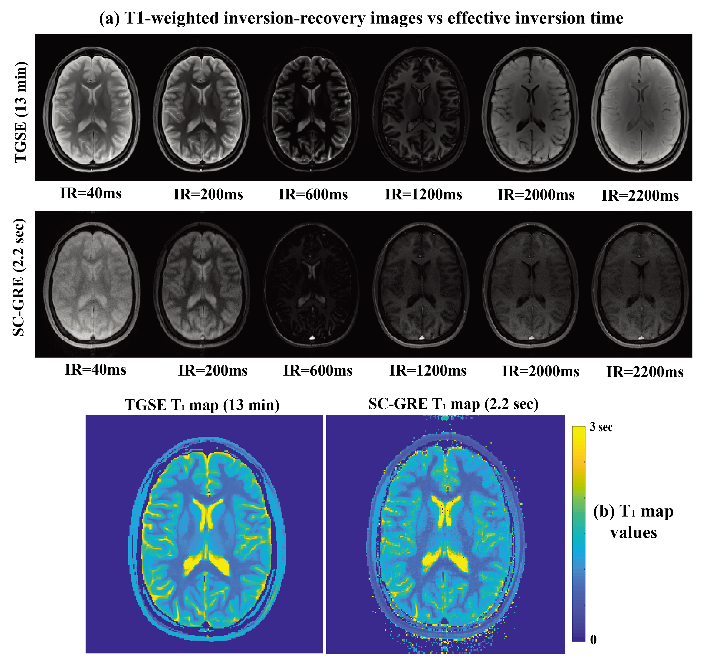
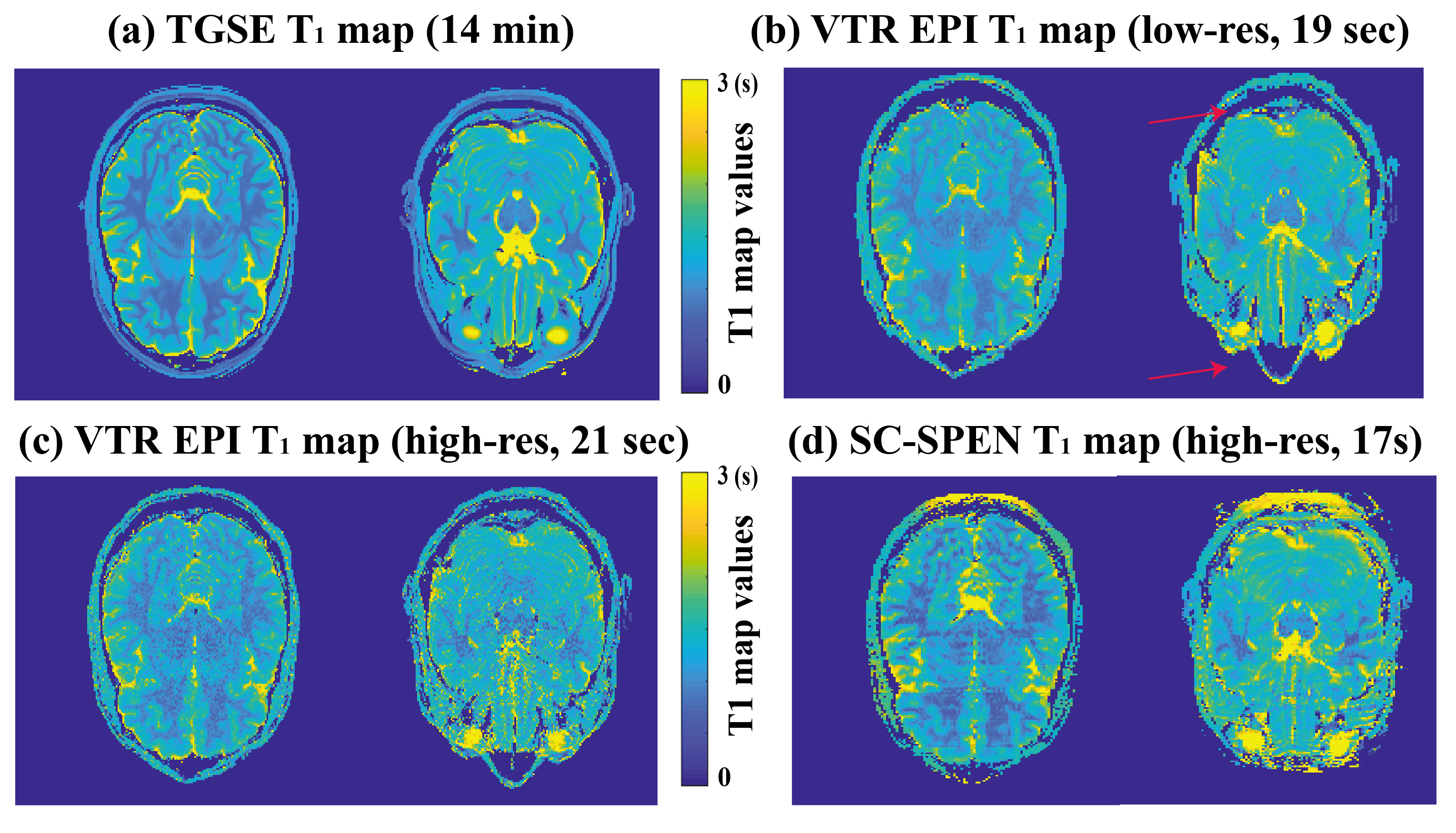
Figure 2 presents in vivo brain T1 maps from TGSE and from SC-GRE (sequence in Fig. 1a). A total of 219 images possessing different phase-encodings and IR weightings were collected every 10ms, and their overall reponse in image and relaxivity spaces reconstructed by the scheme in Eq. (1). At first glance the SC-GRE images do not look identical as their TGSE counterparts (Fig. 2a); however, their translation into T1 maps demonstrate that both data sets contain similar informations content (Fig. 2b) –despite the $$$\geq$$$300-fold difference in the acquisition times they involve.Figure 3 presents a set of fast T1 brain mappings, this time comparing SC SPEN and VTR EPI. The T1 maps arising from both the sequences/processings are consistent with those arising from the TGSE T1 map –while both SPEN and EPI recquiring substantially shorter acquisition times. Still, when collected at comparable resolutions, the SC VTR SPEN T1 maps show higher SNR and considerably fewer distortions than their EPI counterparts. Red arrows in Fig. 3 highlight some of the susceptibility-hit regions in the EPI acquisitions.
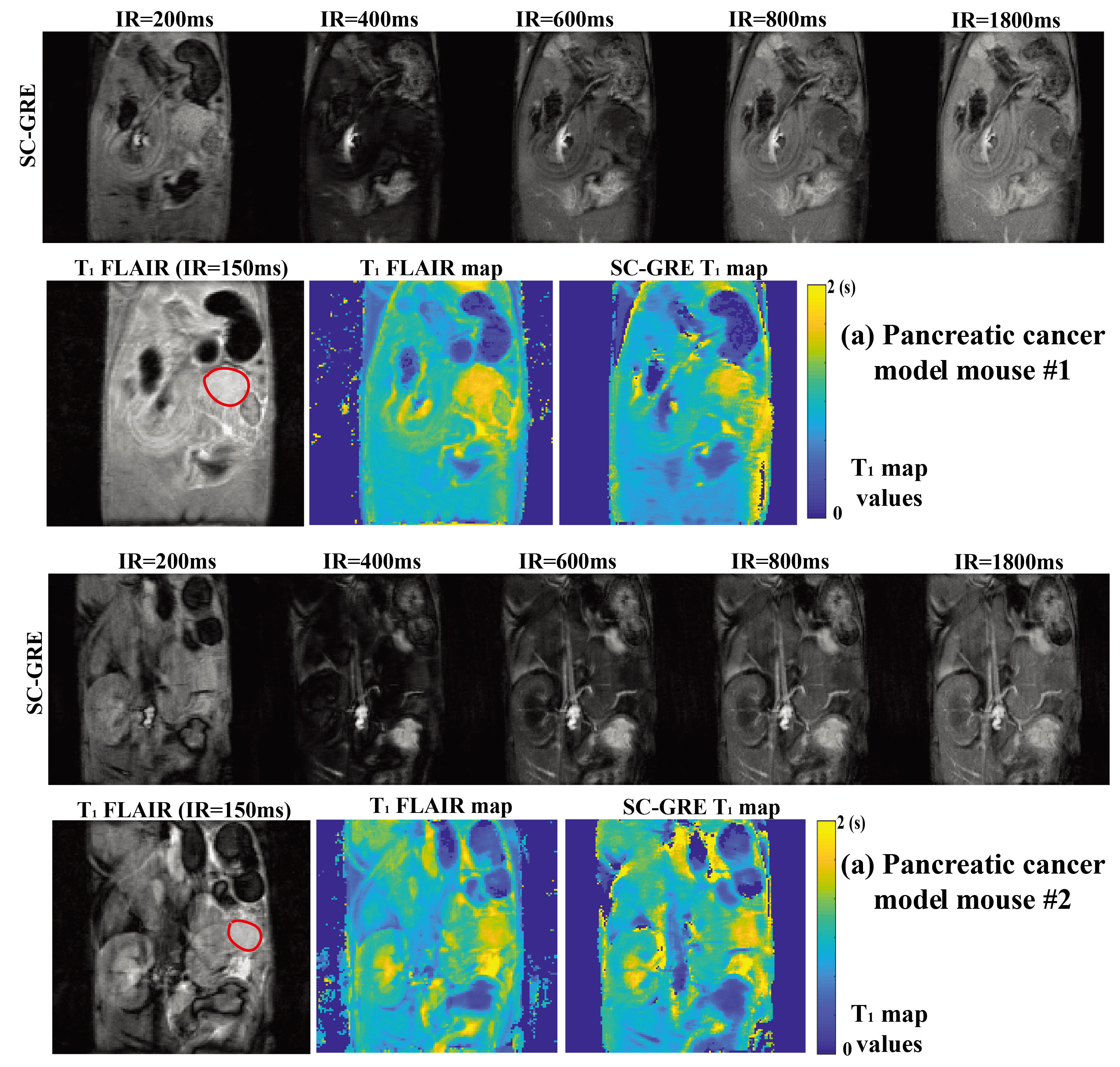
Figure 4 demonstrates the SC sampling approach ability to rapidly map T1 contrasts associated with pancreatic cancer.11 When two mice with such tumors were scanned with SC-GRE and FLAIR, they clearly show the tumors’ higher T1 values, which was reported from literature studies.11 In all cases, the SC-GRE images and maps were consistent with the TGSE data in quality and resolution, despite involving ca. 120$$$\times$$$ shorter acquisition times.
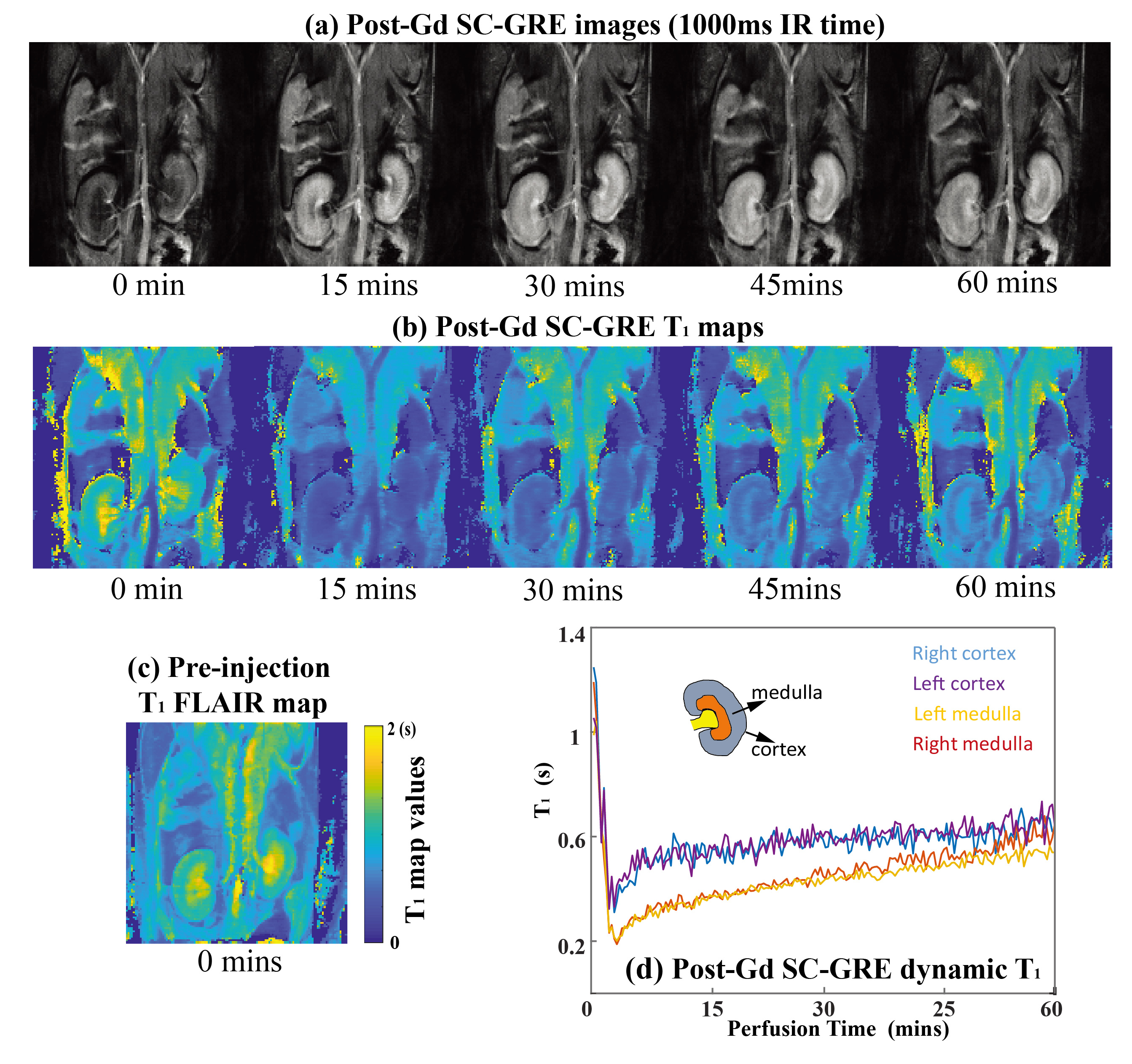
The proposed approaches also allow one to follow dynamic changes, something that is useful for elucidating functional or perfusion characteristics in contrast-enhanced imaging. This is illustrated in Figure 5, where a contrast agent was administered to a live anesthetized mouse, and attention focused on kidney imaging. IR SC-GRE could generate dynamic multi-contrast images and T1 maps with a time resolution of 5s. The kidneys evidence a clear, region-specific T1 shortening during the wash-in of the contrast bolus, and a subsequent T1 lengthening with its washout (Figure 5d). The first post-injection T1 map thus obtained is in agreement with a pre-injection TGSE T1 map collected in 10 mins (Figure 5c).
Conclusion
A method capable of providing rapid multi-contrast T1 images and T1 maps from a few scans/ a single scan, was introduced and demonstrated for a variety of sequences and platforms. The method can supply valuable information on pathology in reduced scanning times, as well as a dynamic T1 mapping information of great use in quantitative DCE MRI assessments.Acknowledgements
We are grateful to D. Preise, K. Sasson and A. Scherz for the pancreatic model. This work was funded by the Israel Science Foundation (grants 2508/17 and 965/18), by the Kimmel Institute of Magnetic Resonance (Weizmann Institute), by China Scholarship Council (CSC) grant 201806310085, and by Israel's Planning and Budget Committee (Lingceng Ma, international student fellowship).References
1. Pedersen H, Kozerke S, Ringgaard S, et al. K-t PCA: Temporally constrained k-t BLAST reconstruction using principal component analysis. Magn. Reson. Med. 2009;62:706–716.
2. Tamir JI, Uecker M, Chen W, et al. T2 shuffling: Sharp, multicontrast, volumetric fast spin-echo imaging. Magn. Reson. Med. 2017;77:180–195.
3. Pfister J, Blaimer M, Kullmann WH, et al. Simultaneous T 1 and T 2 measurements using inversion recovery TrueFISP with principle component-based reconstruction, off-resonance correction, and multicomponent analysis. Magn. Reson. Med. 2019;81:3488–3502.
4. Zhang J, Feng L, Otazo R, et al. Rapid dynamic contrast-enhanced MRI for small animals at 7T using 3D ultra-short echo time and golden-angle radial sparse parallel MRI. Magn. Reson. Med. 2019;81:140–152.
5. Roeloffs V, Uecker M, Frahm J. Joint t1 and t2 mapping with tiny dictionaries and subspace-constrained reconstruction. IEEE Trans. Med. Imaging 2020;39:1008–1014.
6. Bao Q, Solomon E, Frydman L. High ‐ resolution diffusion MRI studies of development in pregnant mice visualized by novel spatiotemporal encoding schemes. 2020:1–13.
7. Solomon E, Nissan N, Furman-haran E, et al. Overcoming Limitations in Diffusion-Weighted MRI of Breast by Spatio-Temporal Encoding. 2015;2173:2163–2173.
8. Solomon E, Liberman G, Nissan N, et al. Robust Diffusion Tensor Imaging by Spatiotemporal Encoding : Principles and In Vivo Demonstrations. 2017;1133:1124–1133.
9. Solomon E, Liberman G, Sklair-levy M, et al. Diffusion-weighted breast MRI of malignancies with submillimeter resolution and immunity to artifacts by spatiotemporal encoding at 3T. 2020:1391–1403.
10. Bao S, Tamir JI, Young JL, et al. Fast comprehensive single-sequence four-dimensional pediatric knee MRI with T2 shuffling. J. Magn. Reson. Imaging 2017;45:1700–1711.
11. Martinho RP, Bao QJ, Markovic S, et al. Identification of variable stages in murine pancreatic tumors by a multiparametric approach employing hyperpolarized 13C MRSI, 1H diffusivity and 1H T1 MRI. NMR in Biomedicine. 2020;e4446.
Figures