0499
Rapid approximate Bayesian $$$T_2$$$ analysis under Rician noise using deep initialization
Jonathan Doucette1,2, Christian Kames1,2, Christoph Birkl3, and Alexander Rauscher1,2,4,5
1UBC MRI Research Centre, Vancouver, BC, Canada, 2Physics & Astronomy, University of British Columbia, Vancouver, BC, Canada, 3Neuroradiology, Medical University of Innsbruck, Innsbruck, Austria, 4Radiology, University of British Columbia, Vancouver, BC, Canada, 5Pediatrics, University of British Columbia, Vancouver, BC, Canada
1UBC MRI Research Centre, Vancouver, BC, Canada, 2Physics & Astronomy, University of British Columbia, Vancouver, BC, Canada, 3Neuroradiology, Medical University of Innsbruck, Innsbruck, Austria, 4Radiology, University of British Columbia, Vancouver, BC, Canada, 5Pediatrics, University of British Columbia, Vancouver, BC, Canada
Synopsis
Rapid approximate Bayesian parameter inference is investigated for $$$T_2$$$ analysis of multi spin-echo signals. We demonstrate that rapid inference using Rician noise distributions is possible using maximum likelihood estimation (MLE) if the MLE procedure is initialized with samples drawn from an approximate Bayesian posterior. This posterior is learned using a conditional variational autoencoder (CVAE) network, trained on exclusively on simulated data. Nevertheless, we show good generalization to three diverse datasets, including improved inference accuracy compared to standard nonnegative least squares-based methods which implicitly assume Gaussian noise.
Introduction
Bayesian parameter estimation methods are robust techniques for quantifying properties of physical systems. In utilising such techniques, one first requires both a physics model and a noise distribution model. In myelin water imaging (MWI)1,2 using a multi spin-echo (MSE) sequence, a useful physics model is the extended phase graph (EPG) algorithm3 with stimulated echo correction4. In peforming $$$T_2$$$ analysis on the measured MSE magnitude signals, signal noise is typically assumed (often implicitly) to be Gaussian. The signal noise is more correctly Rician5 -- Gaussian in both the real and imaginary channels -- but the Gaussian noise assumption is often justified by invoking the high signal-to-noise ratio limit in which Rician distributions approach Gaussian. However, often one is interested in estimating signal properties which are sensitive to noise, such as short $$$T_2$$$ components and the myelin water fraction (MWF). Here, we show that the choice of noise model creates stark differences in parameter estimates using two proposed methods for $$$T_2$$$ analysis under Rician noise: first, using a conditional variational autoencoder (CVAE)6 neural network to directly approximate the Bayesian posterior, and second, through maximum likelihood estimation (MLE). In both approaches, analysis time remains competitive with regularized nonnegative least squares (NNLS), performed using the open-source software package DECAES7.Methods
We consider a two-component EPG model of multi spin-echo MRI time signals$$X_j(t_j=j\cdot\,TE)=\sum_{\ell=1}^{2}A_{\ell}\,EPG(t_j,\alpha,\beta,T_{2,\ell},T_1,TE)$$
where $$$EPG(t,\alpha,T_{2,\ell})$$$ is computed using the EPG algorithm with spin flip angle $$$\alpha$$$, refocusing control angle $$$\beta$$$, and $$$T_{2,1}\leq{}T_{2,2}$$$, with $$$\ell=1,2$$$ the short and long components. This model is a simplification of the multicomponent model4 in DECAES, which uses a fixed spectrum of (default 40) logarithmically-spaced $$$T_{2,\ell}$$$ components, a fixed (default $$$180^\circ$$$) $$$\beta$$$, and a fixed (default $$$1.0s$$$) $$$T_1$$$; $$$TE$$$ is the uniform echo spacing. $$$A_\ell$$$ together with $$$T_{2,\ell}$$$ is referred to as the $$$T_2$$$ distribution. In all cases, the MWF is calculated as $$$\left(\sum_\ell\sigma(T_{2,\ell})\cdot{}A_\ell\right)/\left(\sum_\ell{}A_\ell\right)$$$ where $$$\sigma$$$ is a soft cutoff function; we take $$$\sigma(x)$$$ to be $$$erf(-x)$$$ scaled and shifted such that $$$\sigma(40ms\pm20ms)=0.5\mp0.4$$$.
MLE inference is performed by solving the optimization problem
$$\underset{\theta,\,s}{argmin}\;-\sum_{j=1}^n\log{}P(Y_j\,|\,s\cdot{}X_j(\theta),s\cdot\epsilon)$$
over parameters $$$\theta=(\alpha,\beta,T_{2,1},T_{2,2},A_1,A_2\!=\!1\!-\!A_1,\epsilon)\in\mathbb{R}^{n_\theta}$$$, where $$$\epsilon$$$ is the uniform Rician noise level. An additional scale parameter $$$s$$$ is inferred to account for signal normalization; both simulated- and measured signals $$$X,Y\in\mathbb{R}^n$$$ are normalized to maximum value $$$1$$$. $$$P(x\,|\,\nu,\sigma)=\frac{x}{\sigma^2}\exp(-\frac{x^2+\nu^2}{2\sigma^2})I_0(\frac{x\nu}{\sigma^2})$$$ is the likelihood -- the probability density function of $$$Rice(\nu,\sigma)$$$ evaluated at $$$x$$$ -- and $$$I_0$$$ is the modified Bessel function of the first kind with order zero. Critically, the initial guess $$$\theta_0$$$ is drawn from the CVAE network; this drastically improves both the optimization speed and accuracy, else the MLE optimization may converge to a suboptimal local minimum. Note that unregularized NNLS is equivalent to MLE with uniform Gaussian noise; regularized NNLS (as in DECAES) further imposes a small-amplitude prior on $$$A_\ell$$$.
Approximate Bayesian inference is performed using CVAE networks trained on simulated data $$$\hat{Y}_j\sim{}Rice(X_j(\theta),\epsilon)$$$. CVAE estimators learn to produce samples $$$\hat{\theta}\sim\hat{P}(\theta|\hat{Y})$$$ from an approximation $$$\hat{P}$$$ to the true Bayesian posterior distribution $$$P(\theta|\hat{Y})$$$. The CVAE network $$$\hat{P}$$$ is trained by minimizing $$\mathcal{L}=\mathop{\mathbb{E}}_{\theta\sim{}P_\theta,\,\hat{Y}_j\sim{}Rice(X_j(\theta),\epsilon)}\hat{H}(\theta,\hat{Y})\;\gtrsim\;H(P,\hat{P})\;=\;-\int_\theta{}P(\theta\,|\,\hat{Y})\log\hat{P}(\theta\,|\,\hat{Y})$$ over the parameters of $$$\hat{P}$$$, where $$$\hat{H}$$$ -- where $$$\mathbb{E}$$$ is the expectation over batches of $$$\theta,\hat{Y}(\theta)$$$ pairs -- is an upper bound (in expectation) of the cross entropy $$$H$$$ between the true posterior $$$P$$$ and approximate posterior $$$\hat{P}$$$. $$$P_\theta$$$ is a prior distribution over the parameters of interest. See figure 1 for the CVAE model architecture, which mirrors that of6, but with multilayer perceptrons replaced with multiheaded self-attention blocks, inspired by recent work in image classification8. The CVAE was trained using the ADAM optimizer with initial learning rate $$$10^{-4}$$$, with learning rate drops on plateaus of the validation loss by $$$\sqrt{10}$$$ until convergence
Three diverse CPMG datasets are used for validation of this method on real data; see table 1 for scan details.
Results and Discussion
We perform three experiments to investigate the proposed method.First, we perform inference on simulated signals $$$\hat{Y}$$$ generated from fixed $$$\theta$$$ and compare the accuracy of the estimated $$$\hat{\theta}$$$ for DECAES, MLE, and CVAE. Table 2 shows the mean inference error for each parameter, as well as the total inference time for each method, illustrating the speed of the CVAE. MLE and CVAE perform similarly, and achieve lower error values than DECAES in all cases.
Second, we compare the abilities of DECAES and CVAE to distinguish $$$T_2$$$ values as a function of SNR. We set $$$\bar{T}_2=50ms$$$, and let $$$T_{2,short},T_{2,long}=\bar{T}_2/\sqrt{T_{2,ratio}},\bar{T}_2\cdot\sqrt{T_{2,ratio}}$$$, varying $$$T_{2,ratio}$$$ between $$$1.5$$$ and $$$4$$$ and SNR between $$$40$$$ and $$$100$$$. CVAE recovers $$$T_{2,short},T_{2,long}$$$ more accurately in all cases; see figure 2.
Lastly, in figure 3 we visually compare MWF maps generated by each method. The MWF maps generated are consistent among all methods and datasets, with one notable exception: in dataset #3, DECAES underestimates the MWF when using the default refocusing control angle $$$\beta=180^\circ$$$ (bottom left). This is because the 2D multi spin-echo dataset is prone to stimulated echo effects. When setting $$$\beta=150^\circ$$$, consistent results are recovered. CVAE and MLE circumvent this issue entirely by inferring $$$\beta$$$ directly.
Acknowledgements
Natural Sciences and Engineering Research Council of Canada, Grant/Award Number 016-05371, the Canadian Institutes of Health Research, Grant Number RN382474-418628, the National MS Society (RG-1507-05301). J.D. is supported by NSERC Doctoral Award and Izaak Walton Killam Memorial Pre-Doctoral Fellowship. A.R. is supported by Canada Research Chairs 950-230363.References
- Alex Mackay, Kenneth Whittall, Julian Adler, David Li, Donald Paty, and Douglas Graeb. Invivo visualization of myelin water in brain by magnetic resonance. Magnetic Resonance inMedicine, 31(6):673–677, 1994.
- Kenneth P Whittall and Alexander L MacKay. Quantitative interpretation of NMR relaxationdata. Journal of Magnetic Resonance (1969), 84(1):134–152, August 1989.
- J Hennig. Multiecho imaging sequences with low refocusing flip angles. Journal of MagneticResonance (1969), 78(3):397–407, July 1988.
- Thomas Prasloski, Burkhard Mädler, Qing-San Xiang, Alex MacKay, and Craig Jones. Appli-cations of stimulated echo correction to multicomponent T2 analysis. Magnetic Resonance inMedicine, 67(6):1803–1814, 2012.
- S. O. Rice. Mathematical Analysis of Random Noise. Bell System Technical Journal, 23(3):282–332, 1944.
- Hunter Gabbard, Chris Messenger, Ik Siong Heng, Francesco Tonolini, and RoderickMurray-Smith. Bayesian parameter estimation using conditional variational autoencoders forgravitational-wave astronomy. arXiv:1909.06296 [astro-ph, physics:gr-qc], September 2019.
- Jonathan Doucette, Christian Kames, and Alexander Rauscher. DECAES - DEcomposition andComponent Analysis of Exponential Signals. Zeitschrift Fur Medizinische Physik, May 2020.
- Alexey Dosovitskiy, Lucas Beyer, Alexander Kolesnikov, Dirk Weissenborn, Xiaohua Zhai,Thomas Unterthiner, Mostafa Dehghani, Matthias Minderer, Georg Heigold, Sylvain Gelly,Jakob Uszkoreit, and Neil Houlsby. An Image is Worth 16x16 Words: Transformers for Im-age Recognition at Scale. arXiv:2010.11929 [cs], October 2020.
Figures
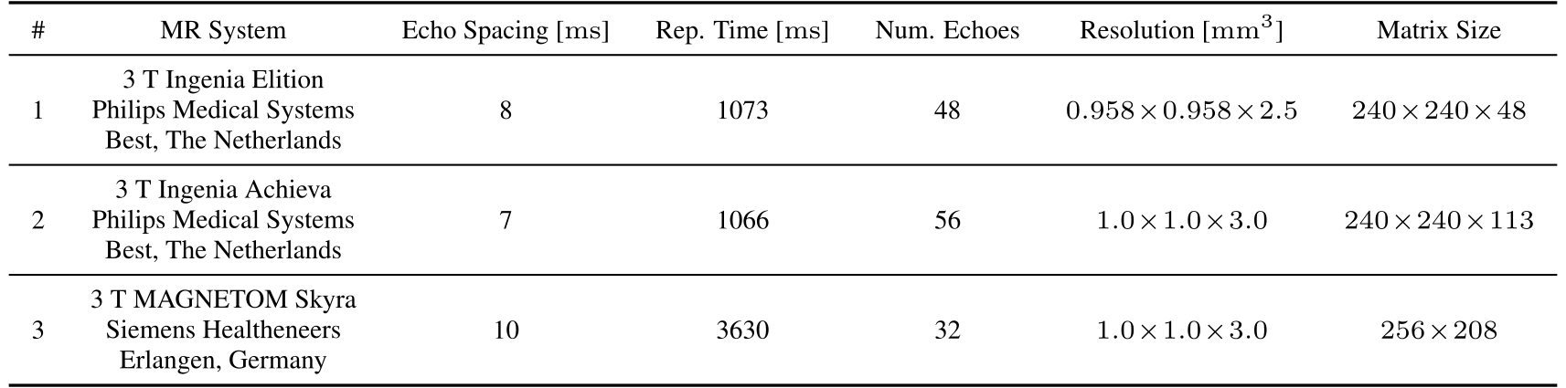
Table 1: MRI datasets used for method validation. Datasets #1 and #3 are acquired in axial orientation; dataset #2 sagitally. Reconstructed resolution is shown. All echo times are uniformly spaced with the shown spacing.
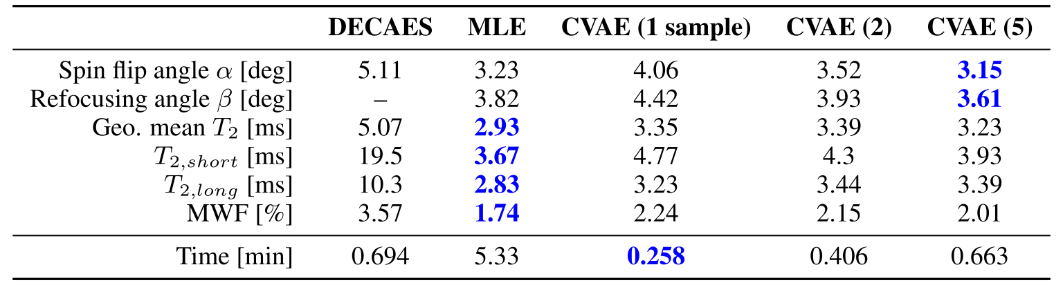
Table 2: Mean absolute error values over inferred $$$\hat{\theta}$$$ for each method. CVAE ($$$n$$$) indicates that $$$\hat{\theta}$$$ is an average over $$$n$$$ samples $$$\hat{\theta}\sim\hat{P}(\theta\,|\,\hat{Y})$$$ from the approximate CVAE posterior $$$\hat{P}$$$.
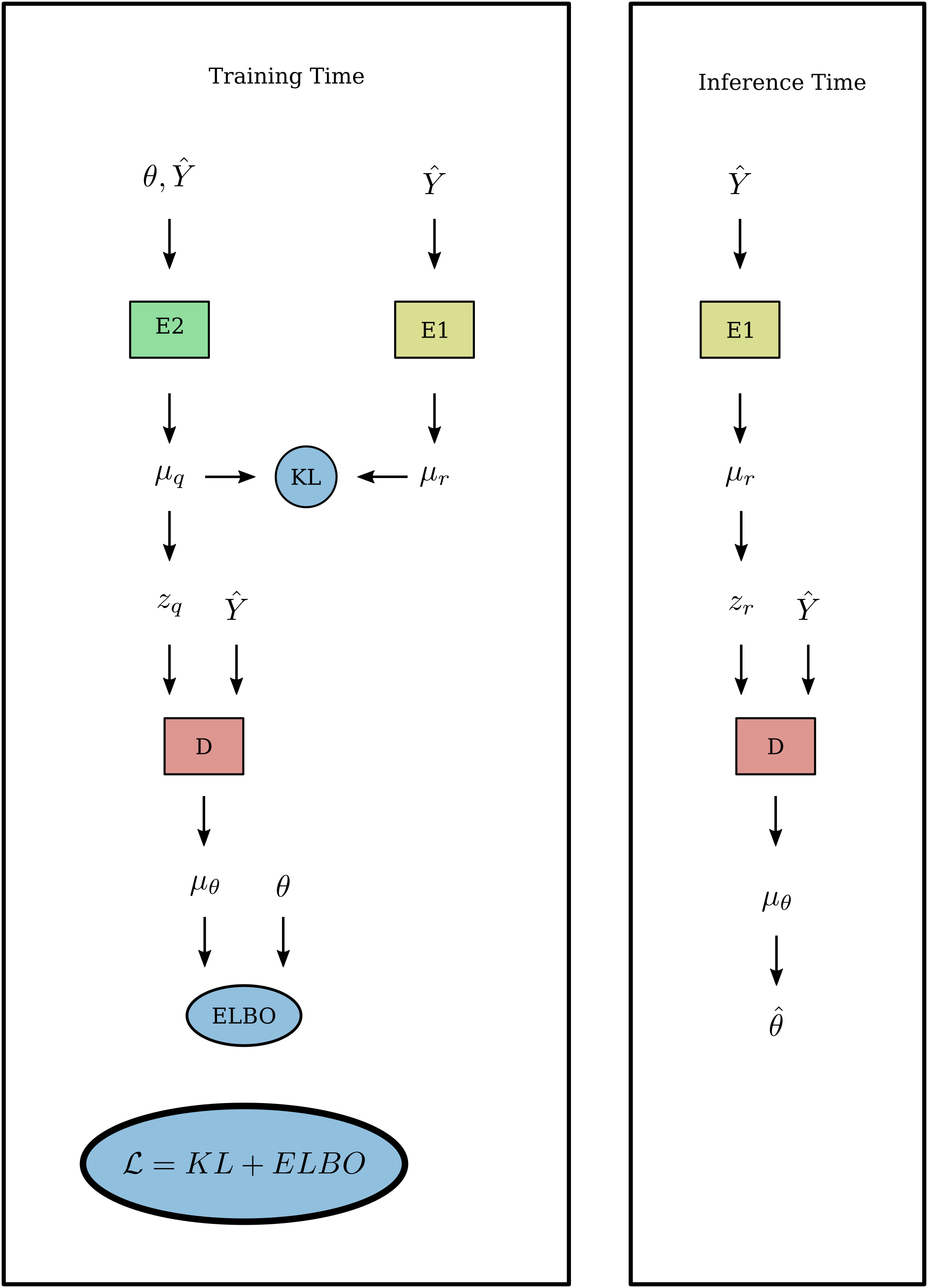
Figure 1: Conditional variational autoencoder network architecture. Encoder networks $$$E_1$$$ and $$$E_2$$$ as well as the decoder network $$$D$$$ implement multiheaded self-attention blocks using 8 heads, input dimension 128, and hidden dimension 256. Intermediate variables $$$\mu$$$ represent parameterizations of multivariate normal distributions; KL is the Kullback-Leibler divergence between the distributions, ELBO is the evidence lower bound.
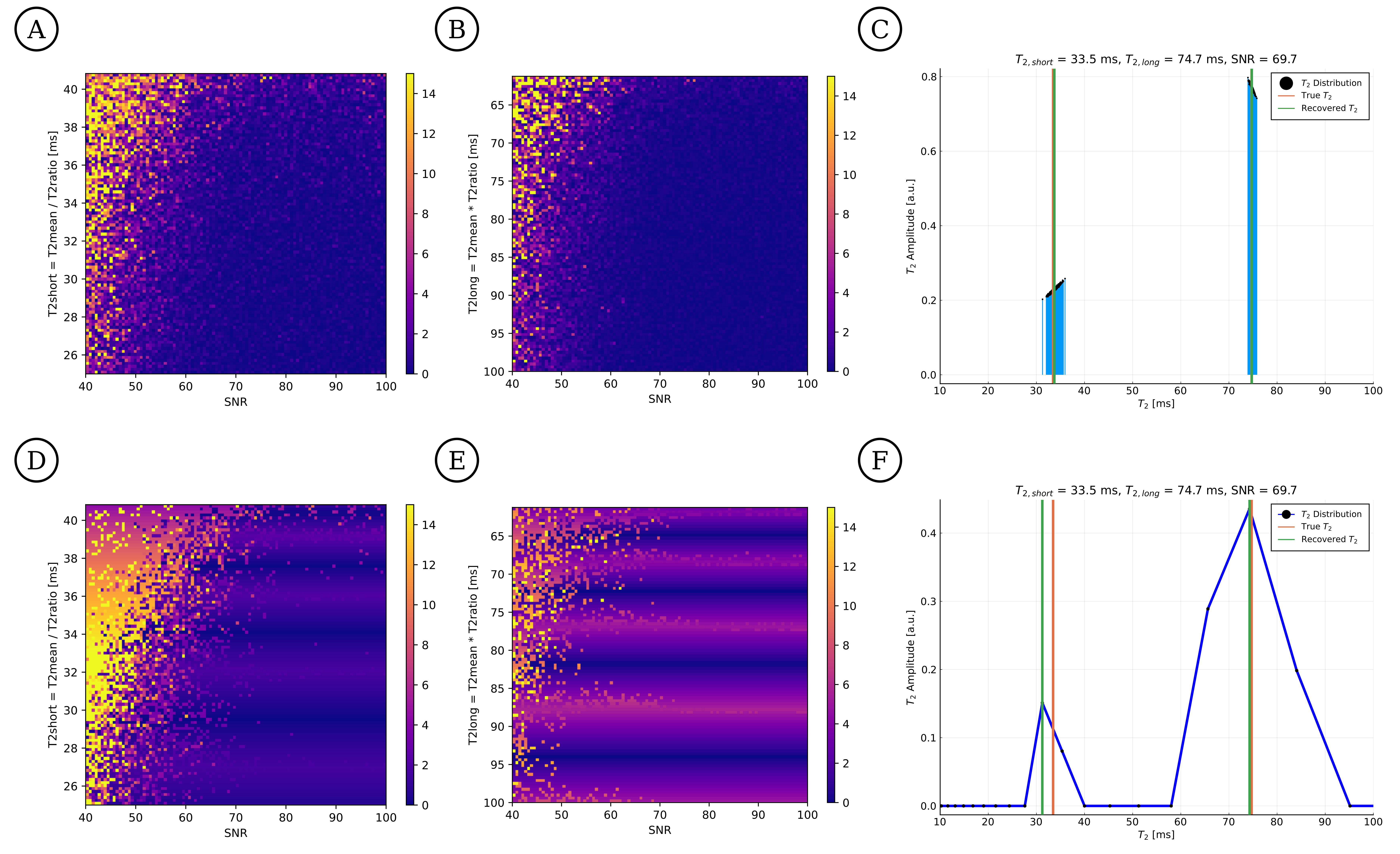
Figure 2: Inference error for CVAE (A,B) and DECAES (D,E) as a function of SNR and $$$T_2$$$ component separation. $$$T_{2,short}$$$ and $$$T_{2,long}$$$ are varied such that $$$T_{2,short},T_{2,long}=\bar{T}_2/\sqrt{T_{2,ratio}},\bar{T}_2\cdot\sqrt{T_{2,ratio}}$$$, where $$$\bar{T}_2=50ms$$$, $$$T_{2,ratio}$$$ varies between $$$1.5$$$ and $$$4$$$, and SNR between $$$40$$$ and $$$100$$$. Example $$$T_2$$$ distributions are shown for CVAE (C) and DECAES (F).
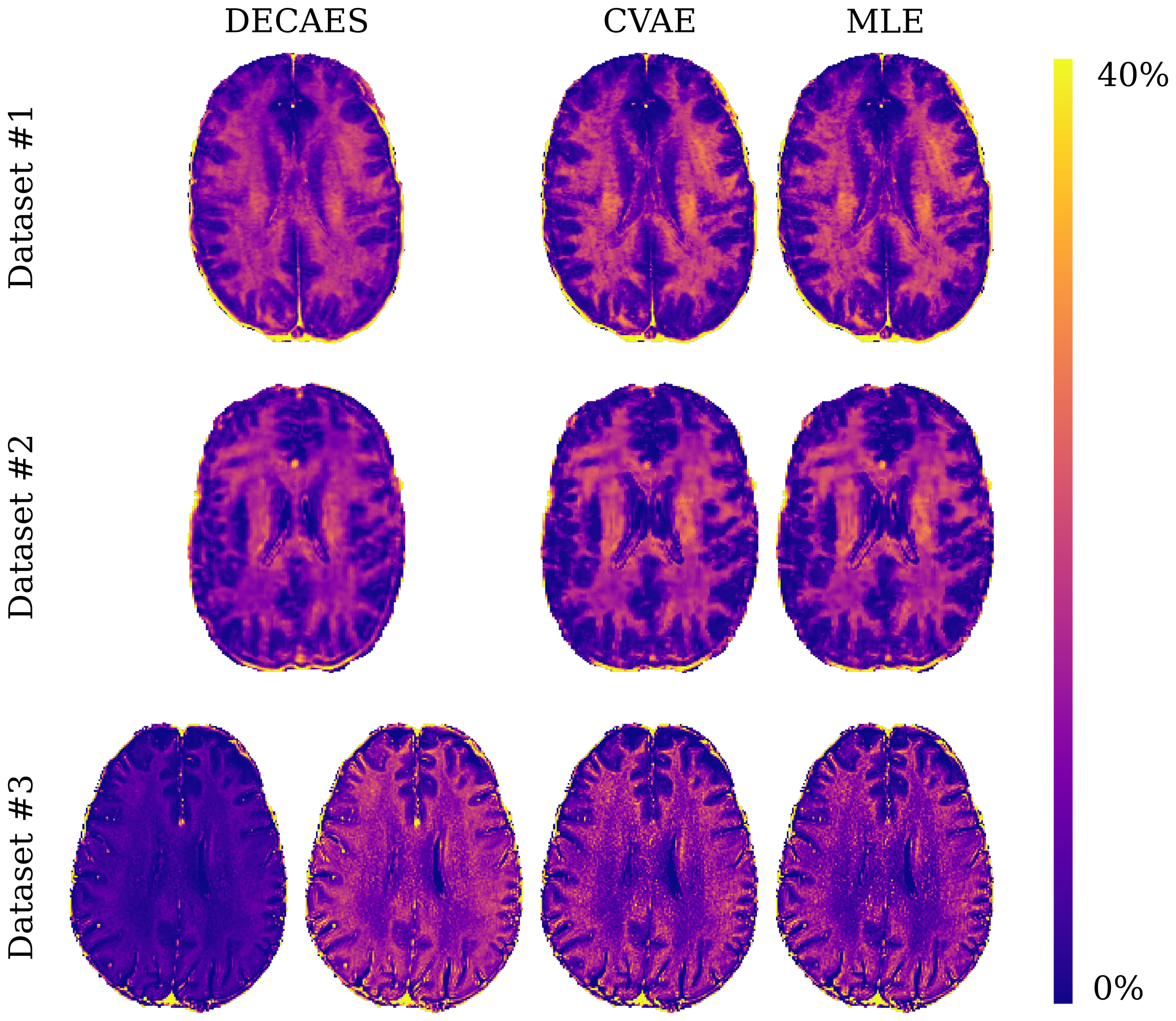
Figure 3: Representative slices of MWF maps resulting from parameter inference using DECAES, MLE, and CVAE. Both CVAE and MLE are able to produce high quality MWF maps for all datasets, despite being trained only on simulated data. In dataset #3, DECAES fails to properly estimate the MWF when using the default refocusing control angle. This can be manually corrected (adjacent), but no such issue occurs for CVAE or MLE which estimate the refocusing control angle directly.