0456
Machine Learning aided k-t SENSE for fast reconstruction of highly accelerated PCMR data1Institute of Cardiovascular Science, University College London, London, United Kingdom
Synopsis
The Machine Learning aided k-t SENSE for the reconstruction of highly undersampled GASperturbed PCMR data is validated. We introduce a modified version of the u-net Convolutional Neural Network (u-net M) that utilises the spatial signal distribution information to improve removal of the MR image magnitude aliases. The high resolution magnitude predictions enable creation of regularisation priors used in the k-t SENSE for the final reconstruction of the PCMR data. 20 patients were scanned in the in-vivo validataion. The technique enabled ~3.6x faster processing than the CS reconstruction with no statistical difference in the measured peak mean velocity and stroke volumes.
Introduction
Highly accelerated real-time Phase Contrast Magnetic Resonance (PCMR)(1) acquisition allows rapid free-breathing blood flow assessments (1-3). Although Compressive Sensing (CS) (4) can resolve the aliasing, its long reconstruction times limit clinical utility. A Machine learning (ML) approach is preferable as the computational load is shifted onto the training stage enabling a significantly shorter processing time. Previously, u-net (5) de-noising models have been successfully applied to image magnitude restoration of undersampled data (6). However, they original implementation works on real numbers and as such is not immediately applicable to PCMR complex data representation, and neglect the data redundancy provided with parallel imaging. To overcome this, we propose an ML aided k-t SENSE two stage reconstruction. In the study we: i) assess the u-net’s ability to produce k-t SENSE regularisation priors, ii) provide the initial validation for quantitative Cardiovascular PCMR and iii) compare the results with CS.Methods
k-t SENSE (7) is formulated as:$$$ \operatorname*{arg\,min}_{\rho_{x,f}}\frac{1}{2} \|E_{x,f→k,t}\rho_{x,f}-y_{k,t}\|_2^2+λ\|M_{x,f}^{-2}\rho_{x,f}\|_2^2 $$$ [1]
$$$E_{x,f→k,t}$$$ – the linear mapping of the acquired k space data ($$$y_{k,t}$$$) to the searched through spatial ($$$x$$$) temporal-frequency ($$$f$$$) space. The regularisation term uses $$$M_{x,f}^{-2}$$$ – the inverse of the expected signal intensity, to restrict the ill-posed system to solutions ($$$\rho_{x,f}$$$) similar to $$$M_{x,f}$$$.
We propose the following estimate of $$$M_{x,f}^2$$$:
$$$M_{x,f}^2=|F_{t→f} U_w (|S^HF_{x→k}^{-1}y_{k,t}|)|^2$$$ [2]
$$$U_w(x)$$$ is a convolutional neural network (CNN) trained to de-alias the magnitudes of the gridded k space data ($$$F_{x→k}^{-1}$$$ – the non-uniform inverse Fourier transform; $$$S^H$$$ – the linear combination of coil data).
Neural Network design
Fig. 1 shows the residual u-net (6) ($$$U_w$$$) and our modified version u-net M ($$$U_w^M$$$). $$$U_w^M$$$ was expanded with the second input of the fully sampled time average magnitude. Due to the memory limitations the input size was fixed to patches of 56x56x56.
Training and data preparation
816 retrospectively gated PCMR magnitudes were processed: median filter, interpolation to the in-vivo data resolution, augmentation with three in-plain rotations (-45o, 0o and 45o); and used for training of the CNNs. The truth images were under-sampled onto the GASperturbed trajectory (4) and regridded to create the corrupted magnitudes. The overlapping patches (56x56x56) were extracted resulting in 122400 paired data sets (split: 80% training and 20% validation).
Reconstruction and in-vivo validation
20 real-time prospectively undersmapled GASperturbed PCMR (4) (FOV: 450x450 mm, TR/TE: 6.7/1.9 ms, temporal resolution: ~26.6 ms, undersampling: 18x) k space sets (270 frames: ~7.2 s) were reconstructed in blocks of 90 (+6 overlapping) with the new two stage technique (Fig. 2).
The magnitude of combined time average and corrupted frames were normalised and separated into 56x56x56 patches for processing by u-nets. The predictions were recombined applying averaging to the overlaps.
To improve SNR the predicted PCMR magnitudes were temporally sorted and low-pass filtered in the temporal frequency space (Tukey filter, cut-off frequency: ~44%). Next, the central part was extracted and used as $$$M_{x,f}^2$$$.
The NVIDIA K40 GPU card was utilised in the processing.
The new technique was compared against the free-breathing Cartesian retrospectively gated sequence (FOV: 350x262 mm, TR/TE: 4.4/1.9 ms, temporal resolution: 18.5 ms) and the CS reconstruction of the same data.
Results
U-net models trainingIn all 20 cases $$$U_w$$$ generated smaller or larger signal abnormalities Fig. 3. These were inadequate for k-t SENSE priors. Consequently, only $$$U_w^M$$$ was used in the in-vivo study.
Feasibility
The CS reconstruction required ~59 s. The ML aided k-t SENSE processing required ~16.6s (gridding: ~3.9s, $$$U_w^M$$$: ~9.9s, four iterations k-t SENSE: ~1.9s).
In-vivo flow quantification
In general, the ML aided k-t SENSE generated flow curves were visually sharper than those extracted from the CS results (Fig. 4). In two cases $$$U_w^M$$$ predictions exhibited blurring which propagated to the extracted velocity curves. However, there were no statistical differences (p > 0.2) in peak velocities (Fig. 5) and stroke volumes (p > 0.1) between the tested methods.
Discussion
Algorithms which combine CNN with data consistency layers that are trained together in the end-to-end fashion are known to outperform CS reconstructions (8). However, these approaches require raw k space training data. We present a simpler solution that does not require raw multi-coil training data, but utilises the information about spatial signal distribution. The trained CNN becomes the ‘aid’ to k-t SENSE. Our approach falls under the deep prior learning for inverse problem solving (9, 10). We observed $$$U_w$$$ tended to remove parts of the signal with lower intensity. In two cases this resulted in removal of heart structures for $$$U_w$$$ and the residual temporal blurring in $$$U_w^M$$$. Our work suggests that the conventional u-net model trained on coil combined magnitude cannot generalise to prospectively under-sampled multi-coil data. This rendered the standard u-net inadequate for our problem. By introducing the spatial signal distribution, we were able to substantially improve the CNNs performance and use it successfully to aid the k-t SENSE reconstruction.Conclusion
We have validated the ML aided k-t SENSE reconstruction for the clinically relevant quantitative blood flow assessments. The $$$U_w^M$$$ generated priors enabled artefact suppression on a par with CS with no significant differences in quantitative measures. The timing results suggest the on-line implementation could deliver a substantial increase in clinical throughput.
Acknowledgements
This work was supported in part by British Heart Foundation grant: NH/18/1/33511.
JAS and JMT are funded under the UKRI Future Leaders Fellowship (MR/S032290/1).
JMT is also part funded by Heart Research UK (RG2661/17/20).
References
1. Gatehouse PD, Firmin DN, Collins S, Longmore DB. Real time blood flow imaging by spiral scan phase velocity mapping. Magnetic resonance in medicine : official journal of the Society of Magnetic Resonance in Medicine / Society of Magnetic Resonance in Medicine 1994;31(5):504-512.
2. Hjortdal VE, Emmertsen K, Stenbog E, et al. Effects of exercise and respiration on blood flow in total cavopulmonary connection: a real-time magnetic resonance flow study. Circulation 2003;108(10):1227-1231.
3. Kowalik GT, Steeden JA, Pandya B, et al. Real-time flow with fast GPU reconstruction for continuous assessment of cardiac output. Journal of magnetic resonance imaging : JMRI 2012;36(6):1477-1482.
4. Kowalik GT, Knight D, Steeden JA, Muthurangu V. Perturbed spiral real-time phase-contrast MR with compressive sensing reconstruction for assessment of flow in children. Magnetic resonance in medicine : official journal of the Society of Magnetic Resonance in Medicine / Society of Magnetic Resonance in Medicine 2020;83(6):2077-2091.
5. Ronneberger O, Fischer P, Brox T. U-Net: Convolutional Networks for Biomedical Image Segmentation. Lect Notes Comput Sc 2015;9351:234-241.
6. Hauptmann A, Arridge S, Lucka F, Muthurangu V, Steeden JA. Real-time cardiovascular MR with spatio-temporal artifact suppression using deep learning-proof of concept in congenital heart disease. Magnetic resonance in medicine : official journal of the Society of Magnetic Resonance in Medicine / Society of Magnetic Resonance in Medicine 2019;81(2):1143-1156.
7. Hansen MS, Baltes C, Tsao J, Kozerke S, Pruessmann KP, Eggers H. k-t BLAST reconstruction from non-Cartesian k-t space sampling. Magnetic resonance in medicine : official journal of the Society of Magnetic Resonance in Medicine / Society of Magnetic Resonance in Medicine 2006;55(1):85-91.
8. Aggarwal HK, Mani MP, Jacob M. MoDL: Model-Based Deep Learning Architecture for Inverse Problems. IEEE transactions on medical imaging 2019;38(2):394-405.
9. Zhang L, Zuo W. Image restoration: From sparse and low-rank priors to deep priors [lecture notes]. IEEE Signal Processing Magazine 2017;34(5):172-179.
10. Zhang K, Zuo W, Gu S, Zhang L. Learning deep CNN denoiser prior for image restoration. Proceedings of the IEEE conference on computer vision and pattern recognition; 2017. p. 3929-3938.
Figures
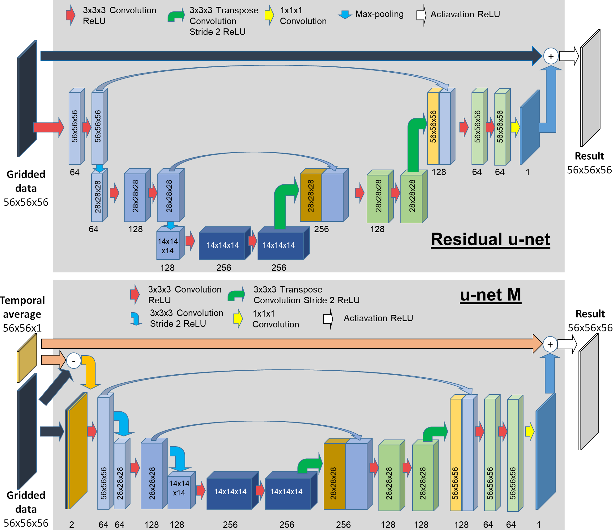
Fig. 1. U-nets architecture.
Three pairs of encoding and decoding units contain two 3D convolutional layers (filter: 3x3x3, ReLU). Max-pooling for $$$U_w$$$ and a stride 2x2x2 in for $$$U_w^M$$$ were used for down-sampling. 3D transpose convolution (stride: 2x2x2, no activation) was used for up-sampling. The last convolution result is added to the undersampled input in $$$U_w$$$ and to the magnitude time average in $$$U_w^M$$$ as a residual update. In $$$U_w^M$$$ the input’s difference is concatenated with the corrupted data to form the input to the first encoding unit.
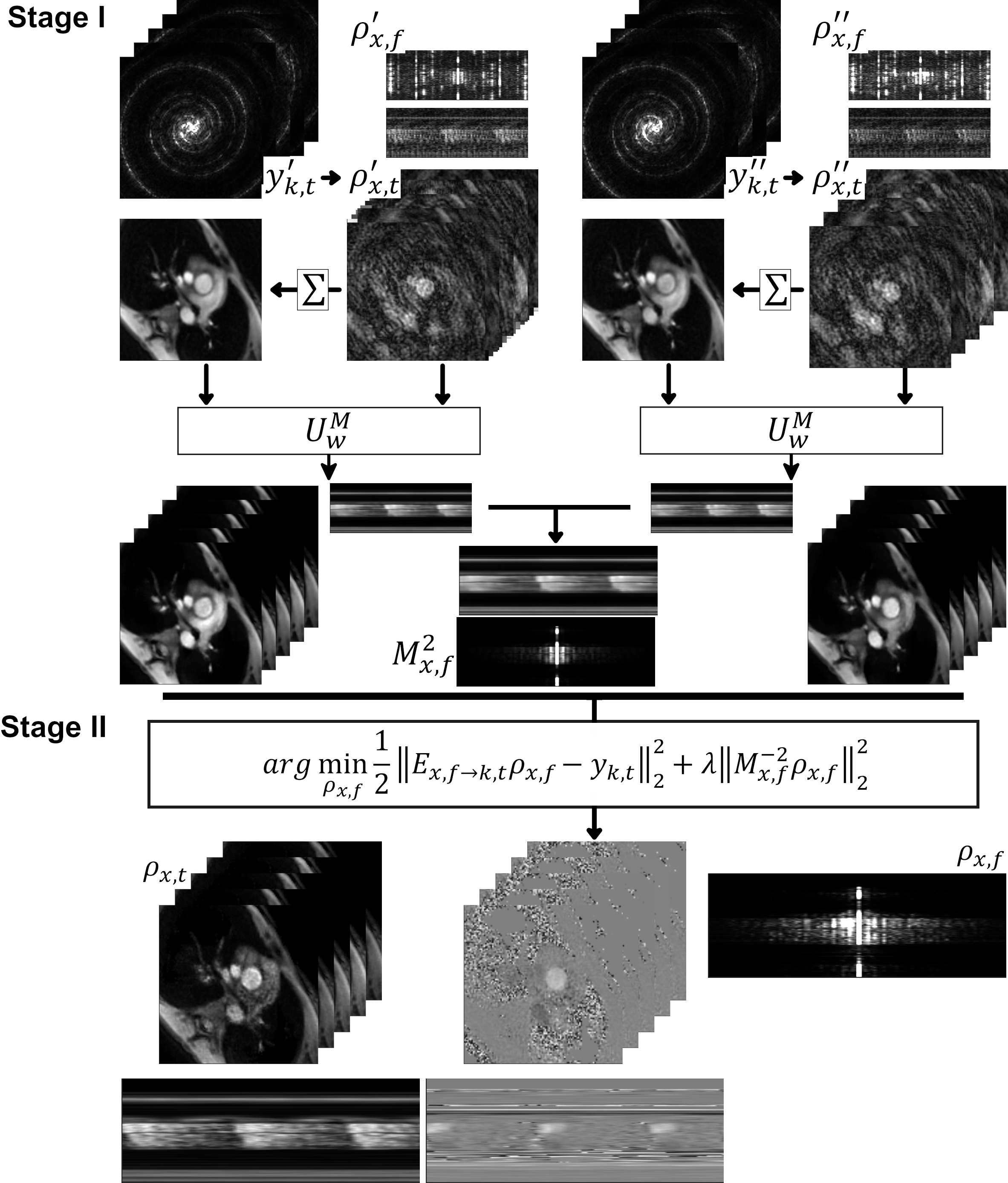
Fig. 2. The ML aided k-t SENSE processing.
Stage I – the $$$M_{x,f}^2$$$ estimation. Both flow encoded ($$$y_{k,t}^{'}$$$) and compensated ($$$y_{k,t}^{''}$$$) data were processed as described [2]. The u-net results were combined for the final x-f signal estimation. Stage II – k-t SENSE: the linear conjugate gradient solver was used to minimise [1] and produce the final PCMR results.
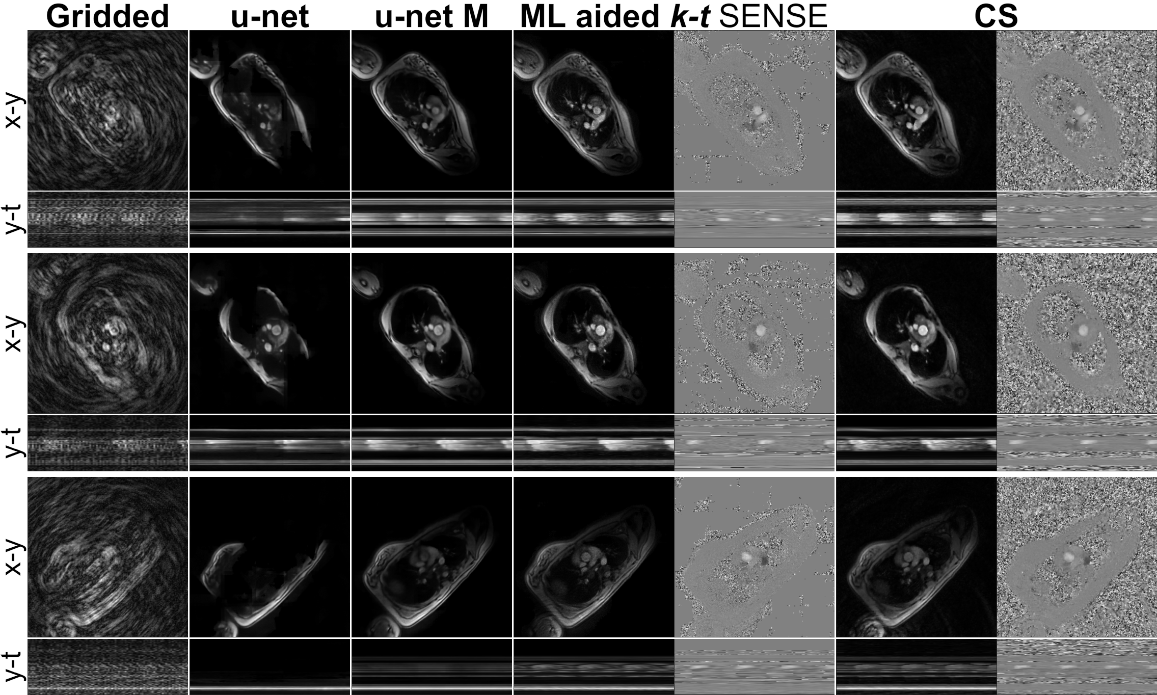
Fig. 3. Imaging results.
$$$U_w$$$ reconstructions presented with smaller or larger artefacts: visible reconstruction patch boundary, signal removal. These are not visible on the $$$U_w^M$$$ results. In two cases $$$U_w$$$ removed heart structures (i.e. the bottom row). In these hard cases temporal blurring can be observed in the $$$U_w^M$$$ results. This had a small effect on the k-t SENSE magnitude results. However, it resulted in blurring of the extracted phase data Fig. 4.
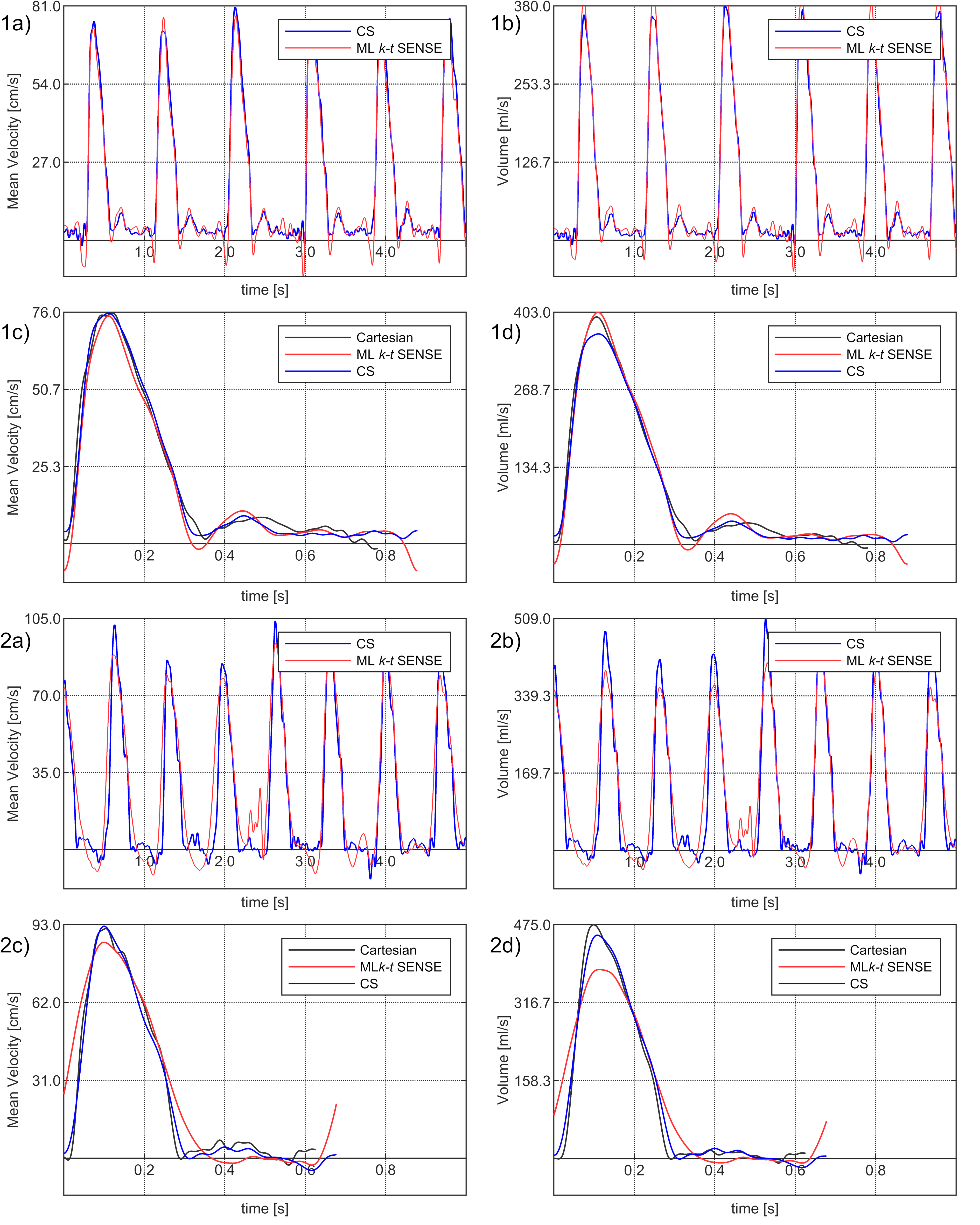
Fig. 4. The flow curves examples.
(1a-d) a comparison of mean velocity (a, c) and volume (b, d) curves extracted from the PCMR results. In general sharper slopes and peaks of the curves in the ML aided k-t SENSE results can be observed. (2a-d) one of the two low signal cases (Fig. 3 – bottom) that resulted in sub-optimal $$$M_{x,f}^2$$$ prediction and blurring of the curves.

Fig. 5. Flow quantification results.
There were no statistical differences (p > 0.2) in peak velocities (Cartesian: 72.4 ± 18.0 cm/s, CS: 72.3 ± 18.6 cm/s and the ML k-t SENSE: 73.2 ± 18.3 cm/s) and stroke volumes (p > 0.1) (Cartesian: 73.2 ± 23.7 ml, CS: 71.4 ± 23.4 ml and the ML k-t SENSE: 72.0 ± 24.1 ml).