0413
Uncertainty Estimation of subject-specific Local SAR assessment by Bayesian Deep Learning1Department of Radiology, University Medical Center Utrecht, Utrecht, Netherlands, 2Computational Imaging Group for MR diagnostics & therapy, Center for Image Sciences, University Medical Center Utrecht, Utrecht, Netherlands, 3Tesla Dynamic Coils BV, Zaltbommel, Netherlands, 4Biomedical Image Analysis, Dept. Biomedical Engineering, Eindhoven University of Technology, Eindhoven, Netherlands, 5Department of Radiotherapy, Division of Imaging & Oncology, University Medical Center Utrecht, Utrecht, Netherlands
Synopsis
Residual error/uncertainty is always present in the estimated local SAR, therefore it is essential to investigate and understand the magnitude of the main sources of error/uncertainty. Last year we presented a Bayesian deep learning approach to map the relation between subject-specific complex B1+-maps and the corresponding local SAR distribution, and to predict the spatial distribution of uncertainty at the same time. The preliminary results showed the feasibility of the proposed approach. In this study, we show its ability to reliably capture the main sources of uncertainty and detect deviations in the MR examination scenario not included in the training samples.
PURPOSE
Local SAR cannot be measured and is usually estimated by off-line numerical simulations. Software tools to perform on-line simulations1 and deep-learning methods2 are being developed. However, the inevitable errors/uncertainties have to be determined to assess appropriate safety factors. Therefore it is crucial to understand the sources of error and uncertainty.Last year we presented a Bayesian deep-learning approach to map the relation between subject-specific complex B1+-maps and the corresponding 10g-averaged SAR (SAR10g) distribution, and to predict the spatial distribution of uncertainty at the same time3.
In deep-learning approaches the sources of uncertainty are generally categorized as either aleatoric or epistemic4,5. Aleatoric uncertainty arises from the natural stochasticity of input data (e.g. due to noisy/imprecise/partial data), and it cannot be reduced. Epistemic uncertainty results from the lack of knowledge (e.g. uncertainty in the model parameters due to a limited amount of training data), and it can be reduced by obtaining additional data.
In this study, we validate the estimated uncertainty by extensive analysis. In addition, the SAR10g assessment method is applied at five other transmit array configurations to verify correct SAR10g and uncertainty prediction for setups that the network was not trained for.
METHODS
We use the same synthetic dataset consisting of complex B1+-maps and corresponding SAR10g distributions2,3 (23×250=5750 data samples) obtained using our database of 23 subject-specific models6 with an 8-fractionated dipole array7,8 for prostate imaging at 7T.To capture both types of uncertainty, we train a convolutional neural network (U-Net) with Monte Carlo dropout5 by minimizing the following loss function4.
$$\mathcal{L}_{Uncertanty} = \frac{1}{N_{voxel}}\sum_{i=1}^{N_{voxel}}\frac{1}{2}\frac{|Ground\texttt{-}Truth_i-Output_i|^2}{\widehat{\sigma}_{Data_i}^2}+\frac{1}{2}\texttt{log}\widehat{ \sigma}_{Data_i}^2$$
The aleatoric data uncertainty $$$\widehat{\sigma}_{Data}$$$ is implicitly learned from this Gaussian log-likelihood loss function. While the epistemic model uncertainty $$$\widehat{\sigma}_{Model}$$$ is estimated by performing fifty stochastic predictions (T=50) with MC dropout for each complex B1+-map. Then, SAR10g ($$$\widehat{\mu}$$$) and uncertainties ($$$\widehat{\sigma}_{Model}$$$ and $$$\widehat{\sigma}_{Model}$$$) are calculated for each voxel i.
$$\widehat{\mu}_i=\frac{1}{T}\sum_{t=1}^{T}Output_{i_t}$$
$$\widehat{\sigma}_{Model_i}=\sqrt{\frac{1}{T}\sum_{t=1}^{T}(Output_{i_t})^2-\left(\frac{1}{T}\sum_{t=1}^{T}Output_{i_t}\right)^2}$$
$$\widehat{\sigma}_{Data_i}=\sqrt{\frac{1}{T}\sum_{t=1}^{T}\widehat{\sigma}_{Data_{i_t}}^2}$$
However, the uncertainties obtained tend to be miscalibrated9. Since we expect $$$\widehat{\sigma}_{Data_i}$$$ and $$$\widehat{\sigma}_{Model_i}$$$ to be correlated, we define the overall predictive uncertainty $$$\widehat{\sigma}_i$$$ as:
$$\widehat{\sigma}_i=\sqrt{s_D^2\widehat{\sigma}_{Data_i}^2+s_M^2\widehat{\sigma}_{Model_i}^2+2s_{DM}(s_D\widehat{\sigma}_{Data_i})(s_M\widehat{\sigma}_{Model_i})}$$
After training, we use a dedicated calibration/validation set (3×10=30 data samples), to determine the scalar calibration parameters $$$s_D$$$, $$$s_M$$$ and $$$s_{DM}$$$ by minimizing the calibration objective over all voxels9.
$$\texttt{arg}\min_{s_D,s_M,s_{DM}}\left(\frac{1}{N_{Calib}}\sum_{i=1}^{N_{Calib}}\frac{1}{2}\frac{|Ground\texttt{-}Truth_i-\widehat{\mu}_i|^2}{\widehat{\sigma}_i^2}+\frac{1}{2}\texttt{log}\widehat{\sigma}_i^2\right)$$
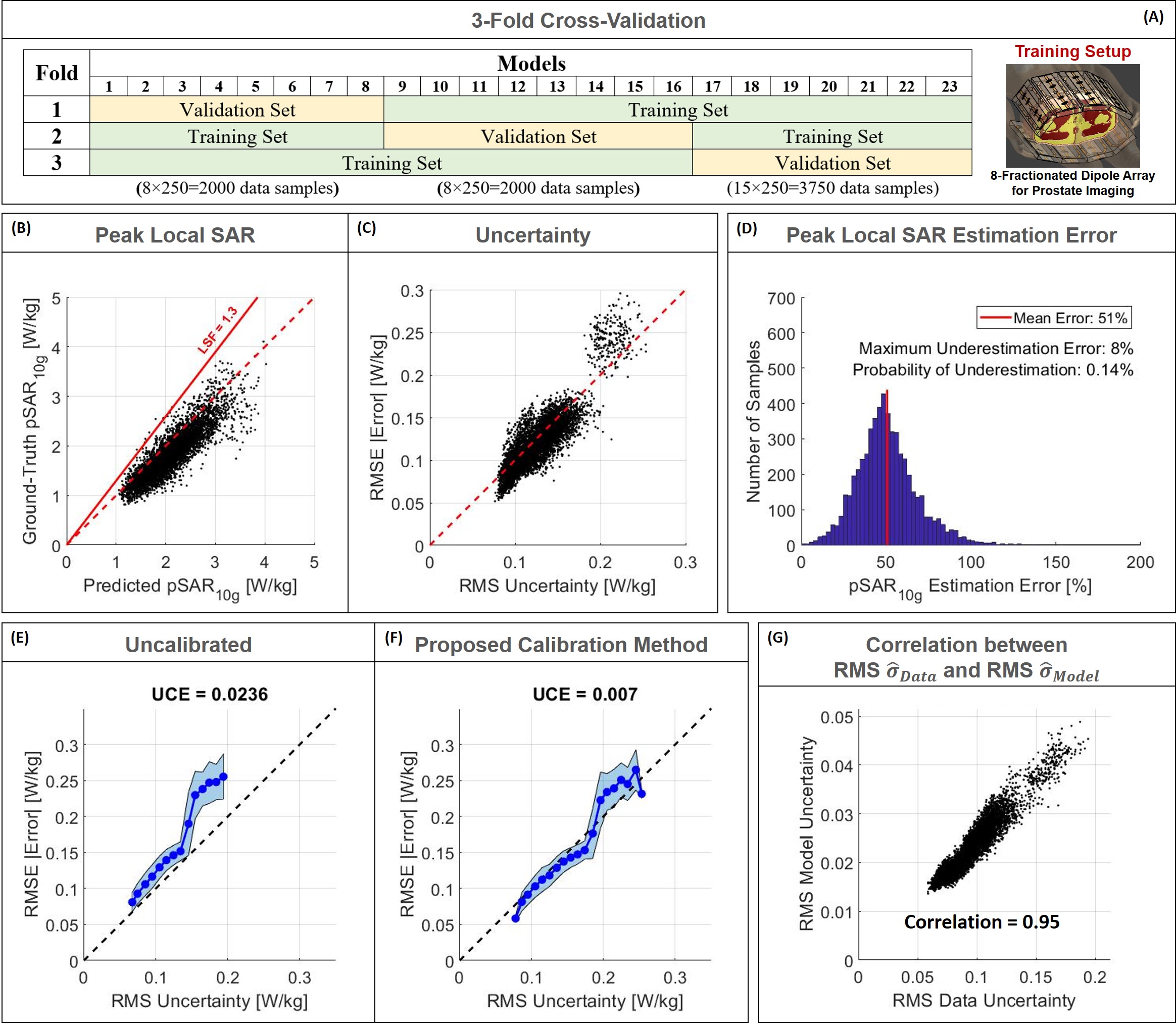
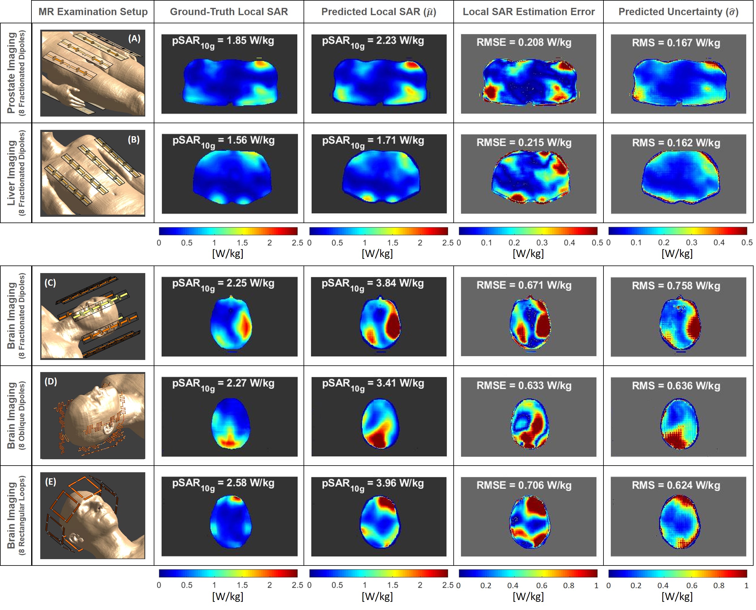
To assess the performance of the proposed approach, a 3-Fold Cross-Validation is performed. In addition, to verify the applicability of the trained network to other transmit arrays that the network has not seen before, the trained network is tested with a dedicated test set containing 2000 data samples obtained for five different MR examination/transmit array setups at 7T (prostate/liver imaging with dipole array and brain imaging with dipole and loop arrays)7,8,10 -12.
RESULTS AND DISCUSSION
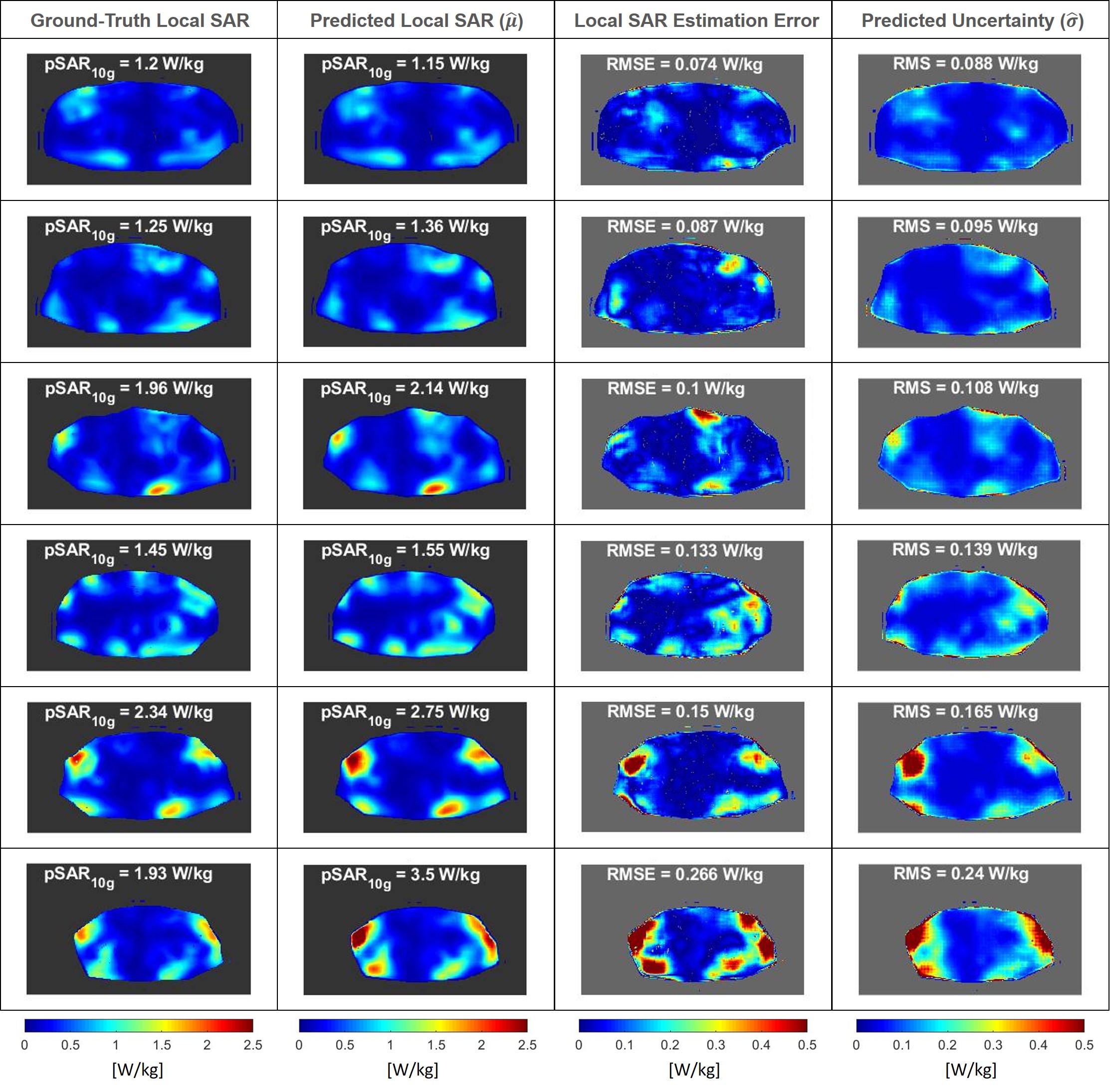
The distributions in Figure 1 show a good qualitative and quantitative match of both SAR10g and uncertainty distributions in six cross-validation examples. The scatter plots in Figure 2 show a good correlation in all cross-validations (A-C).The histogram of the pSAR10g estimation error in Figure 2.D shows a mean overestimation error of 51% with 0.1% probability of underestimation (outperforming our previous deep-learning approach2, mean overestimation error of 56%).
The importance of the calibration of uncertainty contributions is demonstrated by Figure 2.E and 2.F. Without calibration, estimated uncertainty underestimates SAR10g prediction errors whereas proper calibration is able to amend this.
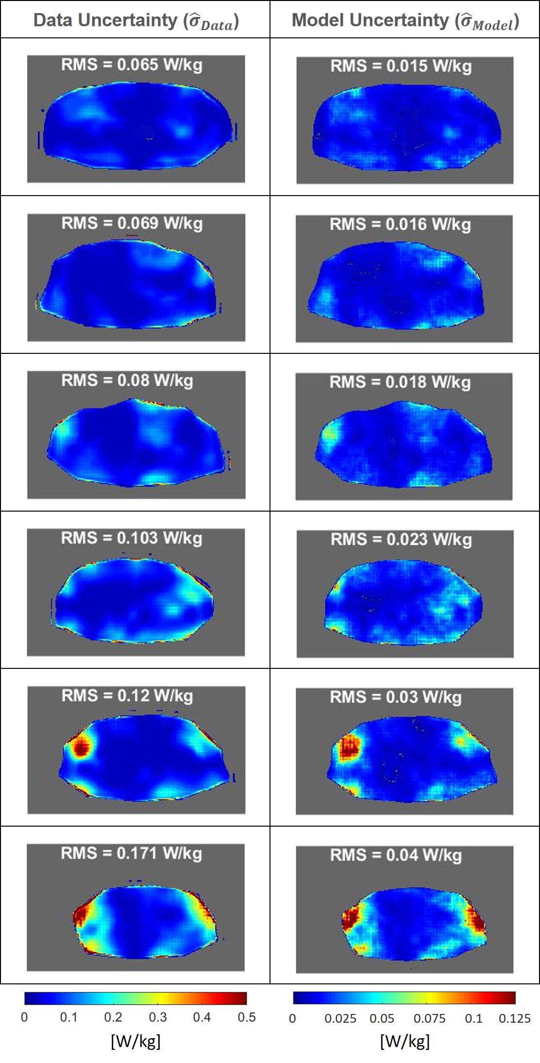
Figure 3 shows the spatial distributions of $$$\widehat{\sigma}_{Data}$$$ and $$$\widehat{\sigma}_{Model}$$$. Although these contributions to uncertainty have been determined independently, they turn out to be highly correlated, which is also indicated by Figure 2.G. Note that because data is used to infer the model parameters, the indicated correlation is to be expected4.
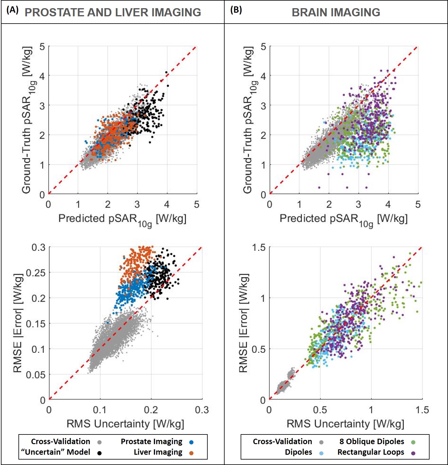
The ability to generalize and predict SAR10g distributions and appropriate levels of uncertainty on out-of-training data is demonstrated by the results in Figures 4 and 5. A quite good qualitative match between the ground-truth and predicted SAR10g distributions are observed visually (Figure 4). The predicted levels of uncertainty are proportional to the SAR10g estimation errors (Figure 5). For prostate and liver imaging, SAR10g predictions are quite accurate and performance similar to the most “uncertain” model in our database (bottom row of Figure 1) is obtained. The head array setups are much less like the prostate setup that the model was trained for which explains the reduced performance for these arrays. However, the poor quantitative performances in SAR10g estimation are accompanied by appropriately large uncertainty predictions (larger for more deviating array setups). These results provide further confidence in the ability of the network to correctly predict uncertainties, even for setups that the network was not trained for.
CONCLUSION
The proposed Bayesian deep-learning approach for SAR10g prediction from complex B1+-maps outperforms the plain deep-learning approach by 9% less overestimation. After appropriate calibration of the model and data uncertainties, the magnitude of predicted uncertainties closely matches the errors between predicted and actual SAR10g predictions. In addition, the network is able to predict SAR10g distributions for array setups that it was not trained for. Arrays that are more dissimilar to the training setup (e.g. head arrays) have larger deviations between predicted and actual SAR10g. It is shown that for these cases the network predicts larger uncertainties demonstrating that also the magnitude of these uncertainties is correctly predicted for non-trained array setups.Acknowledgements
No acknowledgement found.References
1. Villena JF, Polimeridis AG, Eryaman Y, et al. Fast Electromagnetic Analysis of MRI Transmit RF Coils Based on Accelerated Integral Equation Methods. IEEE Trans Biomed Eng. 2016; 63(11):2250-2261.
2. Meliadò EF, Raaijmakers AJE, Sbrizzi A, et al. A deep learning method for image‐based subject‐specific local SAR assessment. Magn Reson Med. 2019;00:1–17.
3. Meliadò EF, Raaijmakers AJE, Maspero M, et al. Subject-specific Local SAR Assessment with corresponding estimated uncertainty based on Bayesian Deep Learning. Proceedings of the ISMRM 29th Annual Meeting, 8-14 August 2020. p. 4195.
4. Kendall A, Gal Y. What Uncertainties Do We Need in Bayesian Deep Learning for Computer Vision?. In: Advances in Neural Information Processing Systems. 2017;5580–5590.
5. Gal Y, Ghahramani Z. Dropout as a bayesian approximation: representing model uncertainty in deep learning. In: Proceedings of the 33rd International Conference on International Conference on Machine Learning, ICML. 2016;1050-1059.
6. Meliadò EF, van den Berg CAT, Luijten PR, Raaijmakers AJE. Intersubject specific absorption rate variability analysis through construction of 23 realistic body models for prostate imaging at 7T. Magn Reson Med. 2019;81(3):2106-2119.
7. Steensma BR, Luttje M, Voogt IJ, et al. Comparing Signal-to-Noise Ratio for Prostate Imaging at 7T and 3T. J Magn Reson Imaging. 2019;49(5):1446-1455.
8. Raaijmakers AJE, Italiaander M, Voogt IJ, Luijten PR, Hoogduin JM, et al. The fractionated dipole antenna: A new antenna for body imaging at 7 Tesla. Magn Reson Med. 2016;75:1366–1374.
9. Laves MH, Ihler S, Fast JF, Kahrs LA, and Ortmaier T. Well-calibrated regression uncertainty in medical imaging with deep learning. In Medical Imaging with Deep Learning, 2020. URL https://openreview.net/forum?id=AWfzfd-1G2.
10. Christ A, Kainz W, Hahn EG, et al. The Virtual Family—development of surface‐based anatomical models of two adults and two children for dosimetric simulations. Phys Med Biol. 2010;55:N23–N38.
11. Restivo M, Hoogduin H, Haghnejad AA, Gosselink M, Italiaander M, Klomp D, et al. An 8-Ch Transmit Dipole Head and Neck Array for 7T Imaging: Improved SAR levels, Homogeneity, and Z-Coverage over the Standard Birdcage Coil. Proceedings of the ISMRMB 33rd Annual Scientific Meeting, Berlin, 29 September-1 October 2016. p. 331.
12. Avdievich NI. Transceiver-Phased Arrays for Human Brain Studies at 7 T. Appl Magn Reson. 2011;41(2-4):483‐506.
Figures