0401
On the use of neural networks to fit high-dimensional microstructure models1Department of Clinical Sciences, Radiology, Lund University, Lund, Sweden, 2Department of Radiology and Nuclear Medicine, St. Olav's University Hospital, Trondheim, Norway, 3Department of Clinical Sciences, Medical Radiation Physics, Lund University, Lund, Sweden, 4Centre for Medical Image Computing and Dept of Computer Science, University College London, London, United Kingdom, 5Radiology, Brigham and Women’s Hospital, Boston, MA, United States, 6Harvard Medical School, Boston, MA, United States
Synopsis
The application of function fitting neural networks in microstructural MRI has so far been restricted to lower-dimensional biophysical models. Moreover, the data sufficiency requirements of learning-based approaches remain unclear. Here, we use supervised learning to vastly accelerate the fitting of a high-dimensional relaxation-diffusion model of tissue microstructure and develop analysis tools for assessing the accuracy and sensitivity of model fitting networks. The developed learning-based fitting pipelines were tested on relaxation-diffusion data acquired with optimal and sub-optimal protocols. We found no evidence that machine-learning algorithms can correct for a degenerate fitting landscape or replace a careful design of the acquisition protocol.
Introduction
Specific features of white matter microstructure can be investigated using biophysical modelling and relaxation-diffusion MRI1,2. However, the increasing complexity of models introduces two challenges: slow non-linear fitting and degenerate parameter estimation3,4. Machine learning has been proposed as a solution5-11, but has only been applied to low-dimensional microstructural models where dense sets of training data are easy to generate7,9,10,12. Using tensor-valued diffusion encoding and correlations with relaxation may resolve the degeneracy in parameter estimation problem13,14, but it is yet unknown if learning-based fitting can replace some or all of such data, thereby simplifying and accelerating the acquisition. In this work, we use neural networks to fit a high-dimensional relaxation-diffusion model of tissue microstructure14, develop strategies for testing the accuracy and sensitivity of the networks, and explore the impact of the acquisition protocol on the network performance.Microstructural Model
We use the model by Lampinen et al.14, who recently extended the “standard model” of WM microstructure2,15 to include the effects of transversal relaxation (T2). The microstructural kernel contains “stick” (S) and “zeppelin” (Z) components with signal fractions fS and 1-fS:$$K=f_\mathrm{S}\exp\left(-bD_\mathrm{I;S}\left(1-b_\Delta\right)\right)\exp\left(-\tau_\mathrm{E}/T_\mathrm{2;S}\right)+\left(1-f_\mathrm{S}\right)\exp\left(-bD_\mathrm{I;Z}\left(1-b_\Delta D_{\Delta;\mathrm{Z}}\right)\right)\exp\left(-\tau_\mathrm{E}/T_\mathrm{2;Z}\right)$$
where τE is the echo-time, and b and bΔ denote the trace and anisotropy of the diffusion-encoding b-tensor (B). The two components have relaxation times T2;S and T2;Z, isotropic diffusivities DI;S and DI;Z, and normalized diffusion anisotropy values DΔ;S=1 and DΔ;Z16. Additionally, the model describe the orientation distribution using 5 spherical harmonics coefficients17. In total, the model features 11 free parameters.
Methods
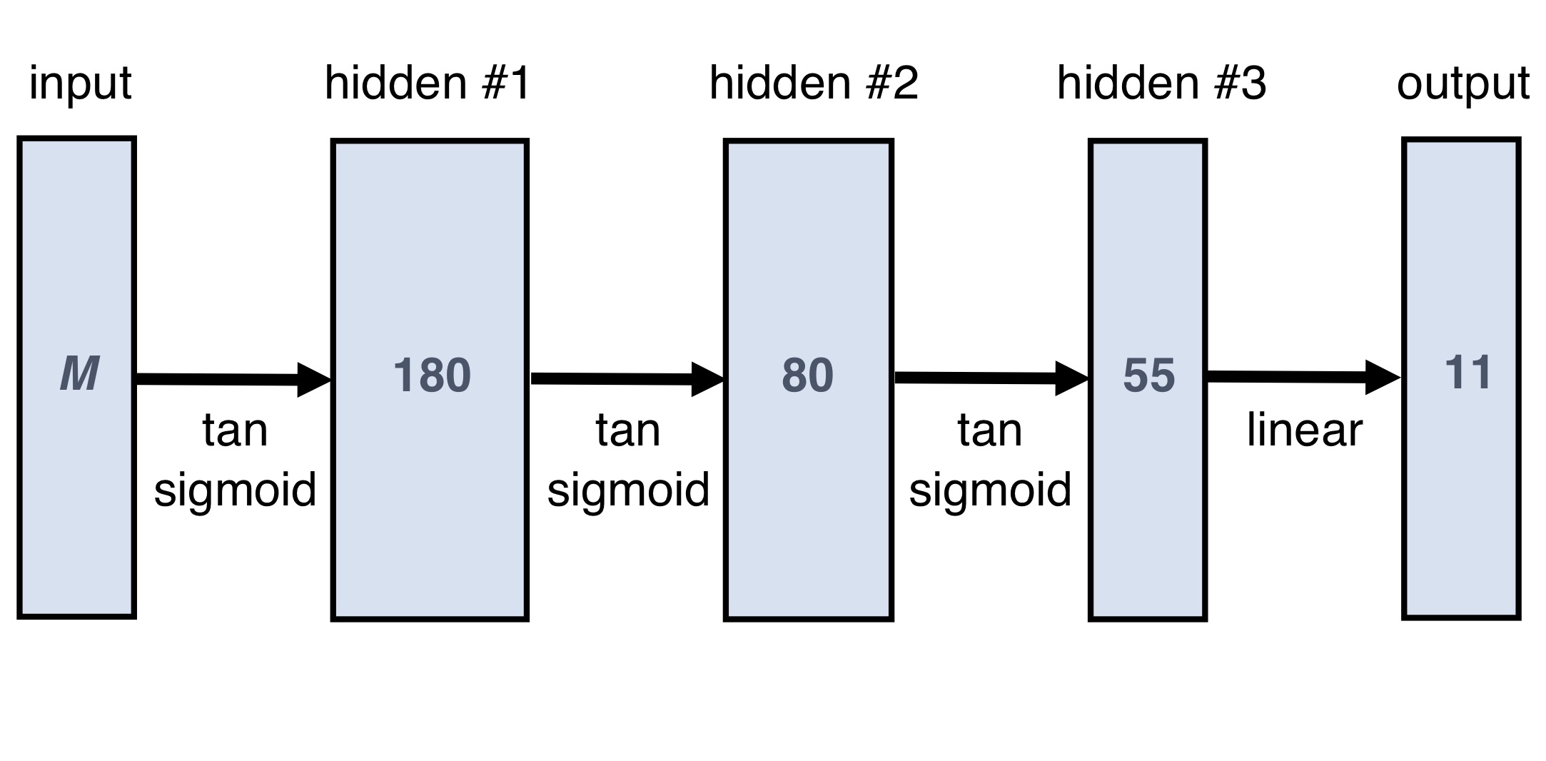
Neural Network design and training: We used a multi-layer perceptron (Fig.1), a network class that can uniformly approximate any continuous function18 and is thus well-suited for non-linear regression problems. The input layer processes M datapoints acquired with different τE and B, while the ouput layer maps to an 11-dimensional model parameter vector.Training was performed on synthetic data, using a scaled conjugate gradient optimiser, a mean-squared error loss function, and validation-based early stopping. The training data was created using two parameter sets:
- 325·103 parameter vectors, obtained by uniform random sampling (munif);
- 175·103 vectors derived from least-squared model fitting to an in vivo brain (mbrain).
The ratio between the number of munif and mbrain vectors was chosen after comparing the performance of networks trained with different relative amounts of munif and mbrain.
Data generation: Synthetic signals were generated from munif and mbrain, using the forward model and one of three (τE,B) acquisition schemes:
- Protocol A, tensor-valued encoding with full relaxation-diffusion-correlation optimised for parameter precision14;
- Protocol B, tensor-valued encoding; relaxation-diffusion-correlations only at low b-values4;
- Protocol C, relaxation-diffusion-correlation scheme optimised for parameter precision, but limited to linear diffusion encoding (bΔ=1)14.
Protocols B and C are known to yield degenerate parameter estimates, while Protocol A is non-degenerate14. All protocols result in acquisition times ~15 minutes.
Distinct datasets and respective networks were generated for each of the above protocols and Rice distributed noise was added to the ground-truth signals. The noise amplitude at b=0 and minimal τE was uniformly sampled from SNR$$$\in$$$[20, 50].
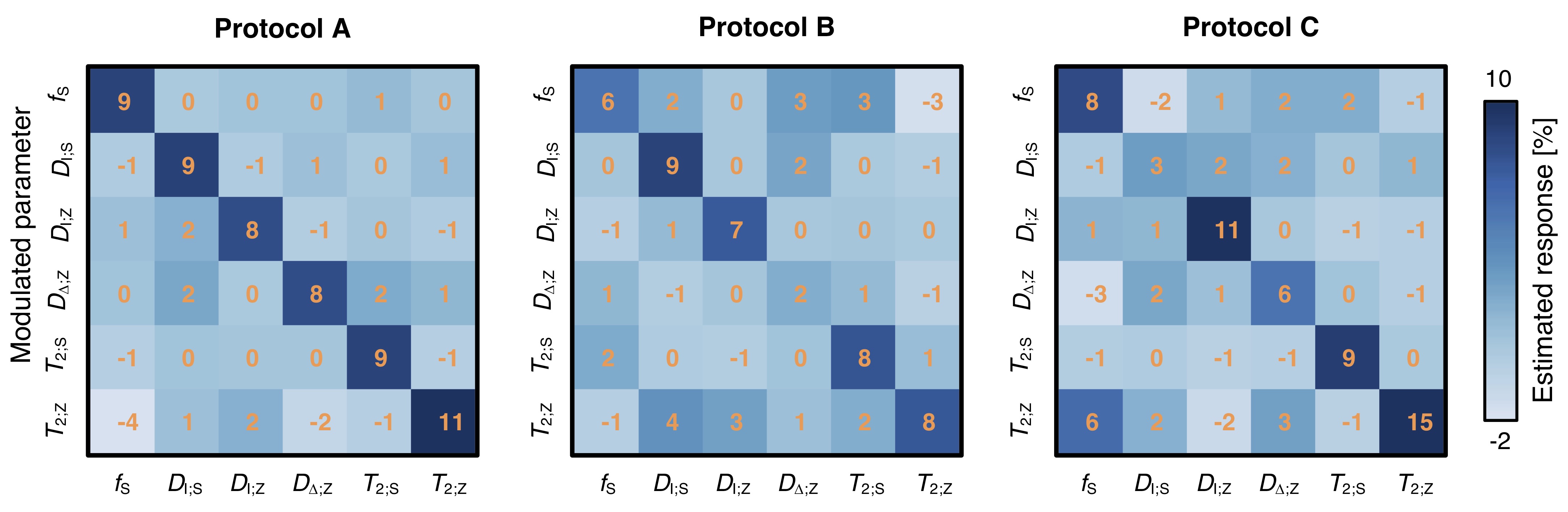
Network evaluation: Networks were deployed on unseen data and compared in terms of normalized root-mean-squared errors (NRMSE), correlation with ground-truth values, and sensitivity to parameter changes. The latter was gauged by sequentially modulating fS,DI;S,DI;Z,DΔ;Z,T2;S,T2;Z by 10% and measuring the response in all parameters.
Results
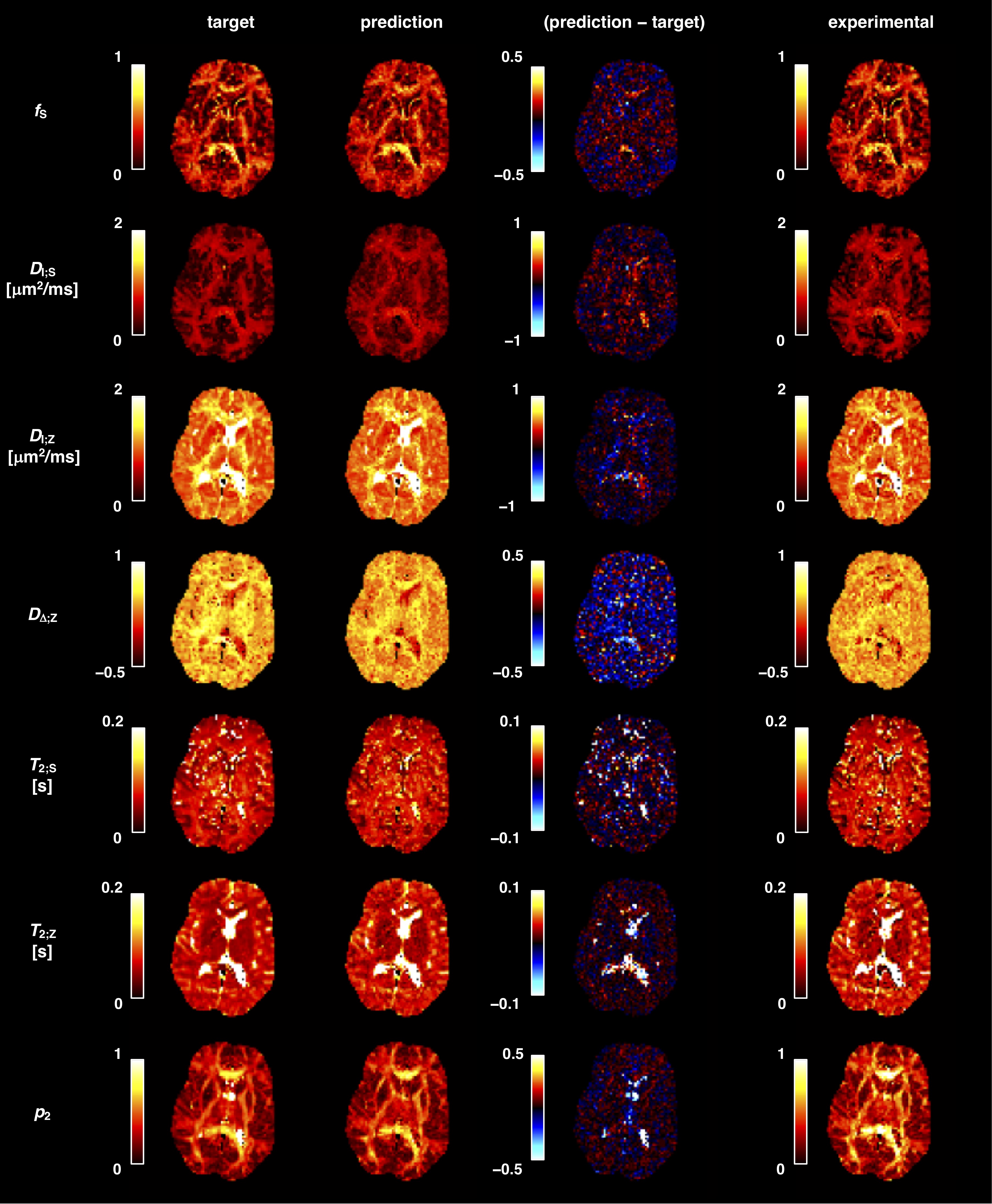
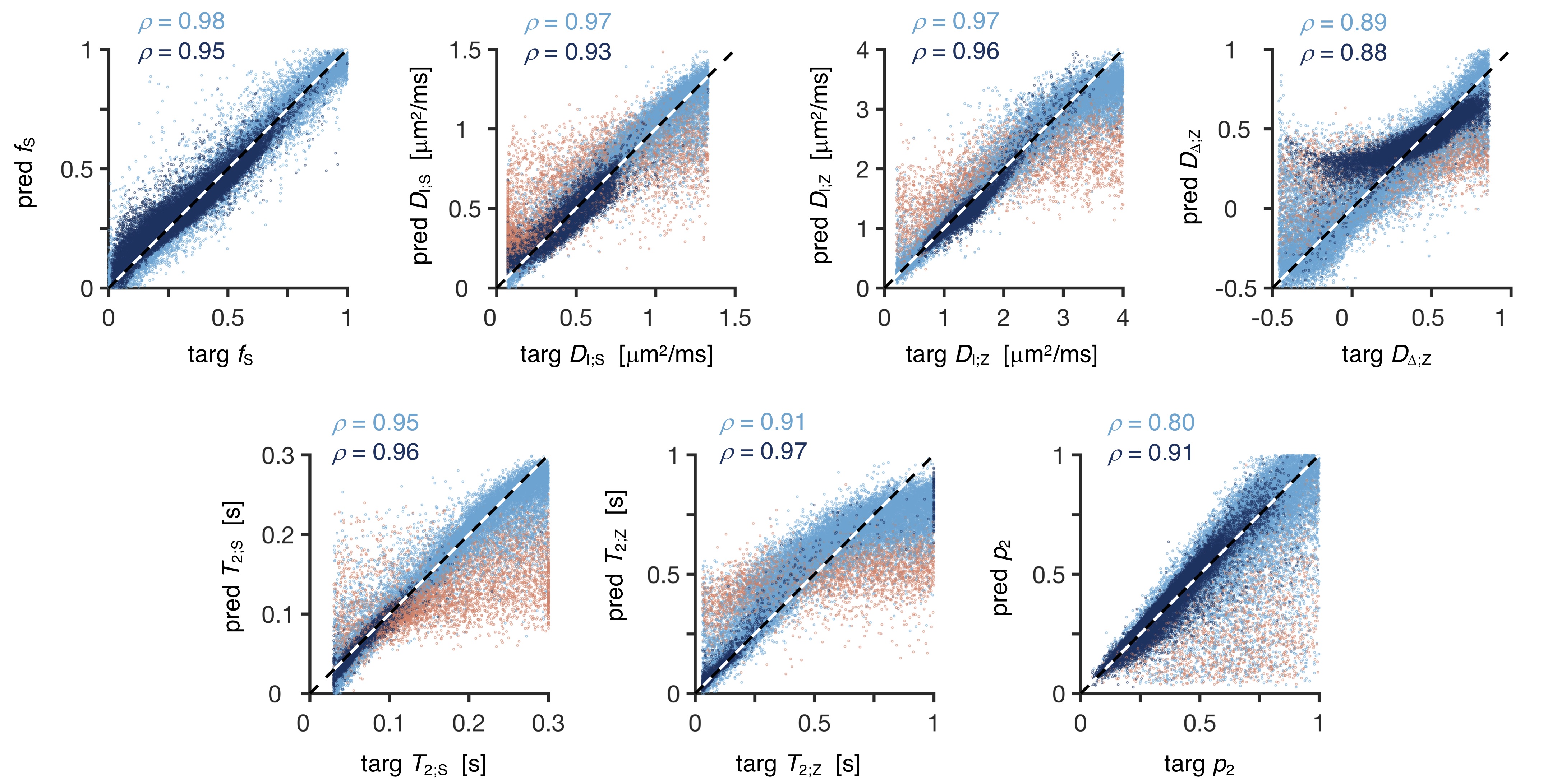
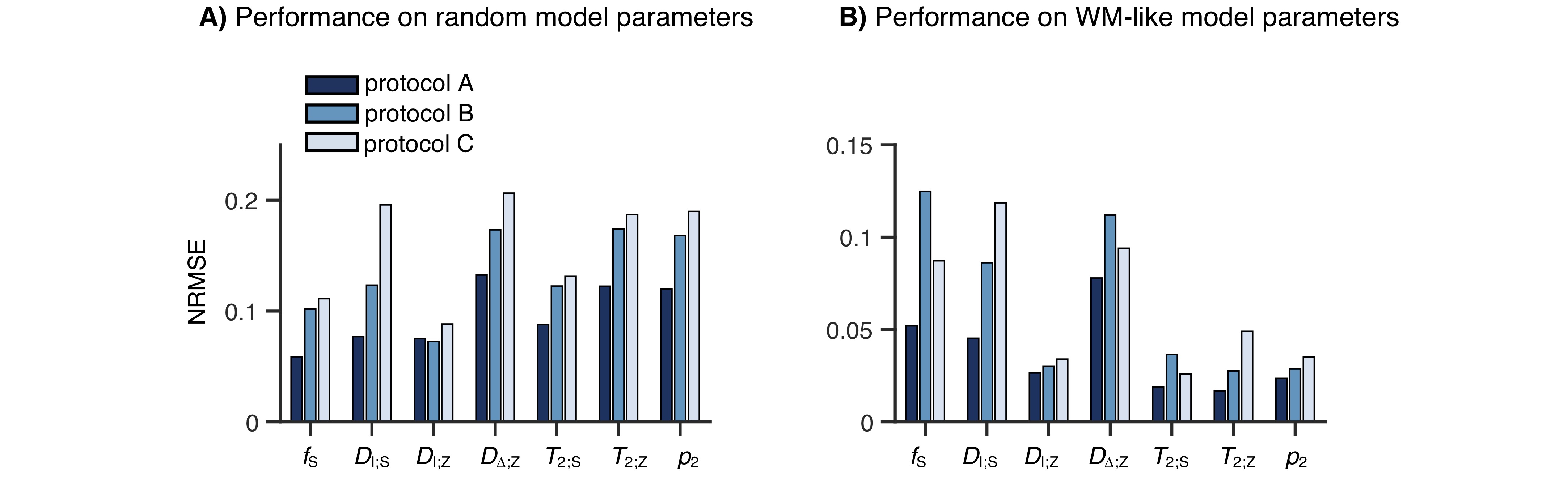
Network-based parameter estimation was ~104 times faster than NNLS fitting on the same PC, and yielded parameter maps in good agreement with each other (Fig. 2). The largest discrepancy was found for DΔ;Z, likely because the signal is insensitive to this parameter below values of 0.519. Figure 3 shows that the network-based estimates correlated well with the ground-truth labels for protocol A, with most parameters yielding linear correlation coefficients above 0.9. Again, the DΔ;Z parameter exhibits poor performance. The same was seen for T2-times that are much longer than the maximal τE. The observed correlations were stronger than those reported in an early learning-based microstructural modelling work7, and equivalent to the correlations reported in more recent studies9,10.Network-based fitting could not ameliorate the known degeneracy in Protocols B and C. Networks based on Protocol A consistently yielded parameter estimates with lower NRMSE (Fig. 4) and stronger correlations to ground-truth values. Sensitivity analysis (Fig. 5) shows that Protocol A is more sensitive to small parameter changes than Protocols B and C, which are oblivious to changes in DΔ;Z and DI;S, respectively.
Discussion & Conclusion
Parameter estimation with high-dimensional microstructural models can be vastly accelerated with function fitting neural networks. Correlation and sensitivity analyses are useful tools for evaluating network performance and for identifying the limitations of learning-based approaches, providing a more rigorous quantitative assessment of parameter-specific accuracy/sensitivity than superficial inspection of machine-learned parameter maps.We found no evidence that probing all dimensions of interest could be replaced, even partially, by the learning-based fitting pipelines. Learning based on inadequate protocols can still generate convincing parameter maps (reproducible, robust, anatomically plausible), but a closer inspection of the network-based estimates reveals both poor accuracy and sensitivity. While deep learning strategies can assist in the design of optimal acquisition protocols20,21, our results suggest that learning-based model fitting cannot by itself substitute for a rich set of data or correct for model degeneracy problems.
Acknowledgements
This work was financially supported by the Swedish Research Council (2016‐03443). J. P. de Almeida Martins gratefully acknowledges support from the Research Council of Norway (FRIPRO Researcher Project 302624) and M. Palombo gratefully acknowledges support from the UKRI Future Leaders Fellowship (MR/T020296/1).
References
1. Nilsson, M., van Westen, D., Ståhlberg, F., Sundgren, P. C. & Lätt, J. The role of tissue microstructure and water exchange in biophysical modelling of diffusion in white matter. Magn. Reson. Mater. Phy. 26, 345-370 (2013).
2. Novikov, D. S., Fieremans, E., Jespersen, S. N. & Kiselev, V. G. Quantifying brain microstructure with diffusion MRI: Theory and parameter estimation. NMR Biomed 32, e3998 (2019).
3. Novikov, D. S., Veraart, J., Jelescu, I. O. & Fieremans, E. Rotationally-invariant mapping of scalar and orientational metrics of neuronal microstructure with diffusion MRI. NeuroImage 174, 518-538 (2018).
4. Lampinen, B. et al. Searching for the neurite density with diffusion MRI: Challenges for biophysical modeling. Hum Brain Mapp 40, 2529-2545 (2019).
5. Golkov, V. et al. q-Space Deep Learning: Twelve-Fold Shorter and Model-Free Diffusion MRI Scans. IEEE Transactions on Medical Imaging 35, 1344-1351 (2016).
6. Nedjati-Gilani, G. L. et al. Machine learning based compartment models with permeability for white matter microstructure imaging. NeuroImage 150, 119-135 (2017).
7. Reisert, M., Kellner, E., Dhital, B., Hennig, J. & Kiselev, V. G. Disentangling micro from mesostructure by diffusion MRI: A Bayesian approach. NeuroImage 147, 964-975 (2017).
8. Bertleff, M. et al. Diffusion parameter mapping with the combined intravoxel incoherent motion and kurtosis model using artificial neural networks at 3 T. NMR in Biomedicine 30, e3833 (2017).
9. Gyori, N. G., Clark, C. A., Dragonu, I., Alexander, D. C. & Kaden, E. in 27th Annual Meeting of the ISMRM (Montreal, Canada, 2019).
10. Palombo, M. et al. SANDI: A compartment-based model for non-invasive apparent soma and neurite imaging by diffusion MRI. NeuroImage 215, 116835 (2020).
11. Grussu, F. et al. Deep learning model fitting for diffusion-relaxometry: a comparative study. bioRxiv (2020).
12. Hill, I. et al. Machine learning based white matter models with permeability: An experimental study in cuprizone treated in-vivo mouse model of axonal demyelination. NeuroImage 224, 117425 (2021).
13. Coelho, S., Pozo, J. M., Jespersen, S. N. & Frangi, A. F. in Medical Image Computing and Computer Assisted Intervention – MICCAI 2019. (eds Dinggang Shen et al.) 617-625 (Springer International Publishing).
14. Lampinen, B. et al. Towards unconstrained compartment modeling in white matter using diffusion-relaxation MRI with tensor-valued diffusion encoding. Magnetic Resonance in Medicine 84, 1605– 1623 (2020).
15. Veraart, J., Novikov, D. S. & Fieremans, E. TE dependent Diffusion Imaging (TEdDI) distinguishes between compartmental T2 relaxation times. Neuroimage 182, 360-369 (2018).
16. Conturo, T. E., McKinstry, R. C., Akbudak, E. & Robinson, B. H. Encoding of anisotropic diffusion with tetrahedral gradients: A general mathematical diffusion formalism and experimental results. Magnetic Resonance in Medicine 35, 399-412 (1996).
17. Jespersen, S. N., Kroenke, C. D., Ostergaard, L., Ackerman, J. J. & Yablonskiy, D. A. Modeling dendrite density from magnetic resonance diffusion measurements. Neuroimage 34, 1473-1486 (2007).
18. Cybenko, G. Approximation by superpositions of a sigmoidal function. Mathematics of control, signals and systems 2, 303-314 (1989).
19. Eriksson, S., Lasic, S., Nilsson, M., Westin, C. F. & Topgaard, D. NMR diffusion-encoding with axial symmetry and variable anisotropy: Distinguishing between prolate and oblate microscopic diffusion tensors with unknown orientation distribution. J Chem Phys 142, 104201 (2015).
20. Pizzolato, M. et al. Acquiring and Predicting Multidimensional Diffusion (MUDI) Data: An Open Challenge in Computational Diffusion MRI, 195-208 (Springer, 2020).
21. Grussu, F. et al. “Select and retrieve via direct upsampling” network (SARDU-Net): a data-driven, model-free, deep learning approach for quantitative MRI protocol design. bioRxiv (2020).
Figures