Introduction

Maximizing spatial resolution and minimizing scan time forces us to deal with noisy and limited data. Thus, efficiently extracting microstructural tissue features of interest from the measurements is crucial. From relaxometry to microstructure MRI, the standard parameter estimation paradigm consists of minimizing an objective function with respect to the parameters of interest given noisy measurements. For its asymptotic benefits, maximum likelihood is a widespread estimator. However, for smooth nonlinear models like the ones we typically see in diffusion MRI¹, parameter estimation is challenging. As the saying goes, `the diffusion signal is remarkably unremarkable'², thus, a typical set of noisy measurements easily becomes overparametrized by the models we use to describe them. This may lead to imprecise or degenerate parameter estimates³. To solve this, constraints⁴, extra assumptions⁵ have been proposed but may lead to bias.

Recently, data-driven approaches from supervised machine learning (ML) have gained popularity due to their ability to quickly solve nonlinear regressions. ML approach is to parametrize the mapping from measurements + noise (realistic model output) to model parameters. Neural networks⁶, random forest⁷, or polynomial regression⁸ have been shown to provide useful results in different MRI applications. However, the influence of the training data on the estimates has been an overlooked ML aspect.

Here, by locally linearizing the model, we analytically derive the optimal mean-squared error (MSE) quality metric of ML parameter estimation as function of SNR. We show that this MSE interpolates between classic max-likelihood quality metric (Cramér-Rao-bound) and the variance of the training set. Remarkably, any `black box' ML regressor approaches this analytical curve. This enables regressor-independent evaluation of data quality and sensitivity to model parameters.

Theory

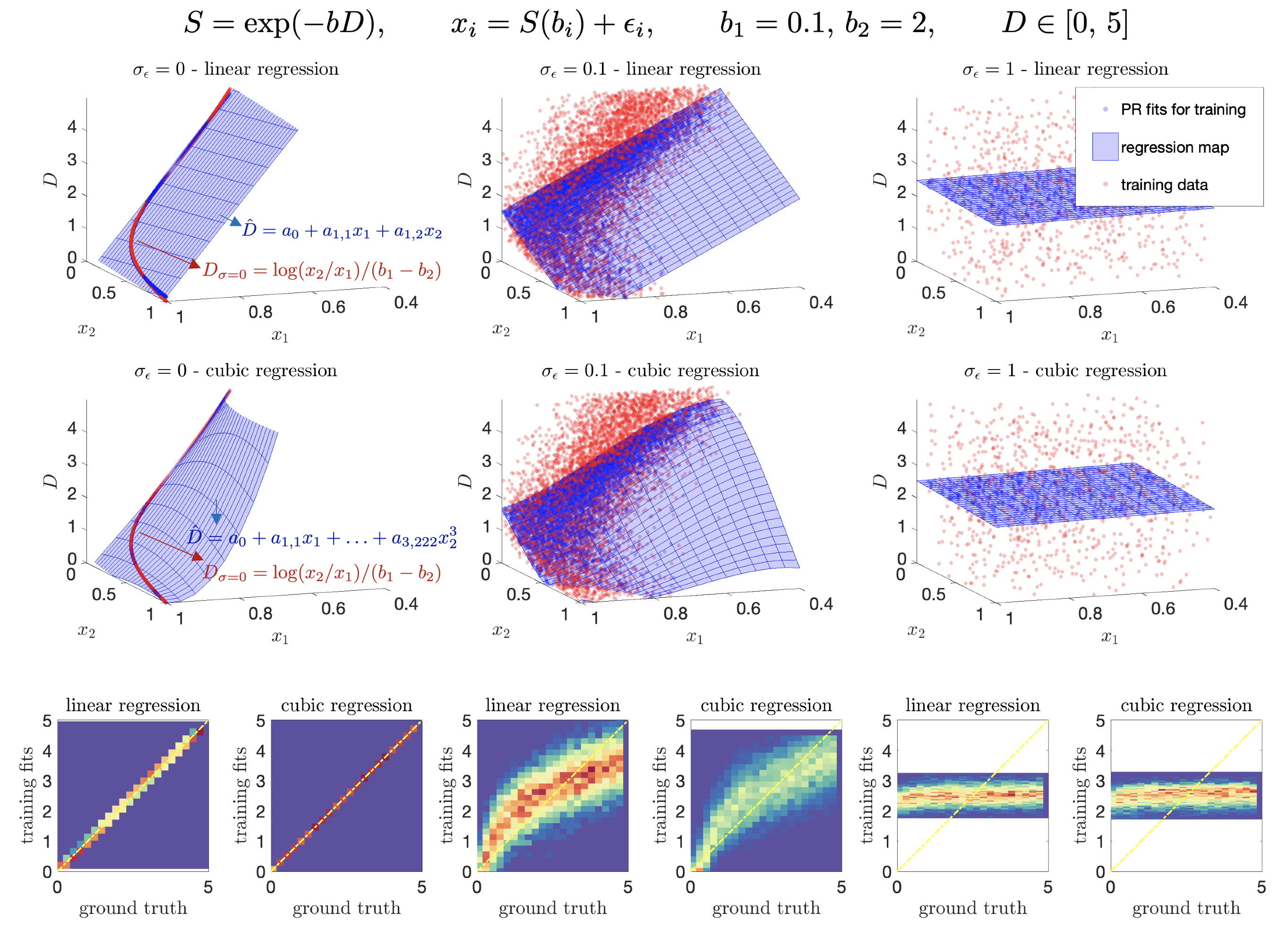
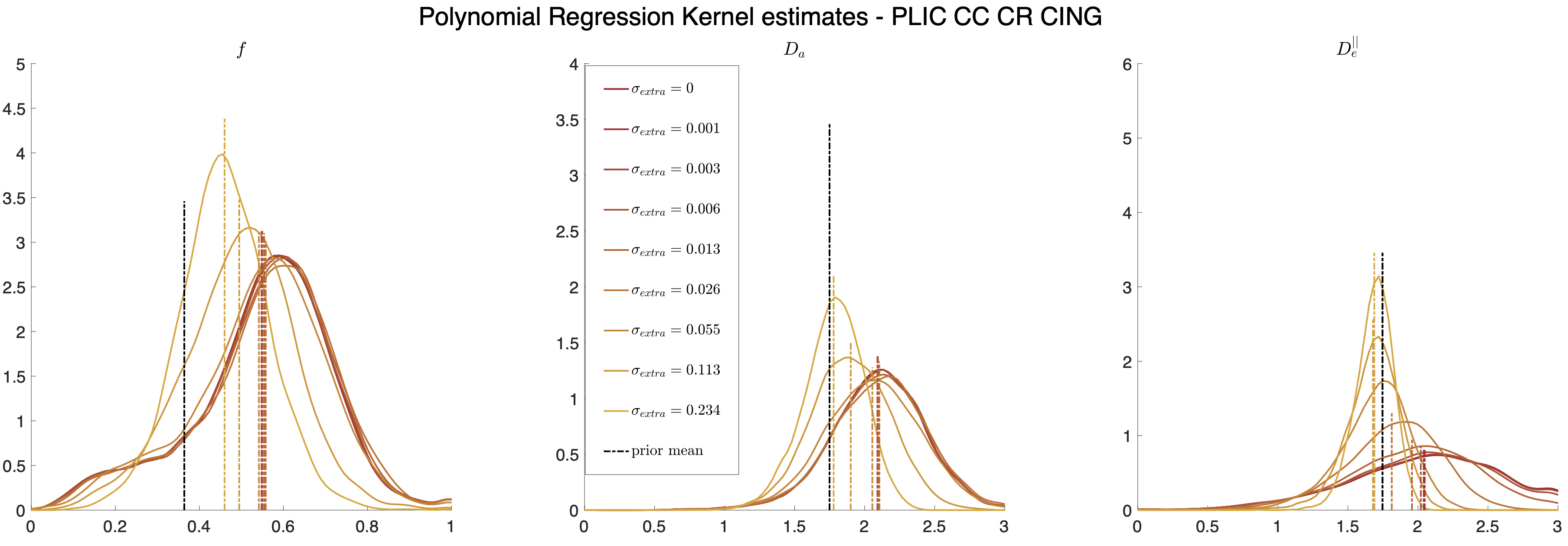
Noise as a regularizer. Supervised ML methods rely on the selection of a prior distribution to generate training data for `learning' the optimal mapping from input features/measurements to parameters. To capture the best mapping for noisy data, noise should be added to the training. However, this has a regularization effect. Figure 1 shows that at different noise levels, the manifold defined by the all the measurements in the training becomes smoothed. Thus, the optimal regression loses complexity. As noise blurs high-order features, the best approximation becomes heavily biased towards the prior distribution that defined such manifold. For extremely low SNR, the optimal regression becomes the expected value of the prior.

Optimal MSE(SNR). Consider a polynomial regression on $$$N$$$ measurements to estimate $$$\theta$$$:
$$\begin{align*}x_{i}&=f_{i}(\theta)+\epsilon_{i},\quad\text{with}\,\quad\,i=1\ldots\,N,\qquad\epsilon\sim \mathcal{N}(0,\sigma),\,\,\epsilon_i\text{ iid}\\\hat{\theta}&=a_0+\sum\limits_{i=1}^N\,a_{1,i}\,x_{i},+\,\text{higher}\,\text{orders},\end{align*}$$
where $$$\hat{\theta}$$$ is our estimator and $$$f(\theta)$$$ our model. In the training, the coefficients of the regression are selected such that they minimize the MSE over noise realizations and training set. For the linear regression, MSE over the training-set
$$\begin{equation*}\mathrm{MSE}_{tr}=\int_{\Theta}d\theta\,\,p\left(\theta\right)\left\langle\left(\hat{\theta}-\theta\right)^{2}\right\rangle= a_{1, i}\,a_{1, j}\left( \overline{ f_i(\theta)\,f_j(\theta)}+\sigma^2\delta_{ij} \right)+a_0^2+\overline{\theta^{2}}+2 \,a_{0}\,a_{1, i}\,\overline{ f_i(\theta)}-2a_{1, i}\,\overline{\theta\,f_i(\theta)}-2 a_{0}\,\overline{\theta},\end{equation*}$$
where angular brackets denote averaging over noise ($$$\langle\epsilon_i\rangle=0,\,\langle\epsilon_i\epsilon_j\rangle=\sigma^2\delta_{ij}$$$), and bar averages over prior $$$p(\theta)$$$. Solving for the regression coefficients minimizing $$$\mathrm{MSE}_{tr}$$$ gives:
$$\begin{equation*}\mathrm{MSE}_{tr}=\operatorname{var}(\theta)-B_{ij}C_{ij},\quad\text{where}\,\,\boldsymbol{B}=(\boldsymbol{\Sigma}+\sigma^2\boldsymbol{I})^{-1},\,\Sigma_{ij}=\overline{f_i(\theta) f_j(\theta)}-\overline{f_i(\theta)}\,\overline{f_j(\theta)},\,C_{ij}=\left(\overline{\theta\,f_i(\theta)}-\overline{\theta}\,\overline{f_i(\theta)}\right)\left(\overline{\theta\,f_j(\theta)}-\overline{\theta}\,\overline{f_j(\theta)}\right).\end{equation*}$$
If we linearly expand $$$f(\theta)\approx\,f(\theta^*)+f'(\theta)\,(\theta-\theta^*)$$$, we can rewrite the above equation as:
$$\begin{equation*}\mathrm{MSE}_{tr}=\frac{\operatorname{var}(\theta)}{1+x_p},\text{where}\,\,x_p=\frac{\operatorname{var}(\theta)}{\operatorname{CRB}(\theta)},\end{equation*}$$
where in this example $$$\operatorname{CRB}(\theta)=I(\theta)^{-1}=(\tfrac{1}{\sigma^2}\frac{d f_i(\theta)}{d \theta}\,\frac{d\,f_i(\theta)}{d \theta})^{-1}$$$. An intuitive meaning for $$$\sqrt{x_p}$$$ is intrinsic SNR.

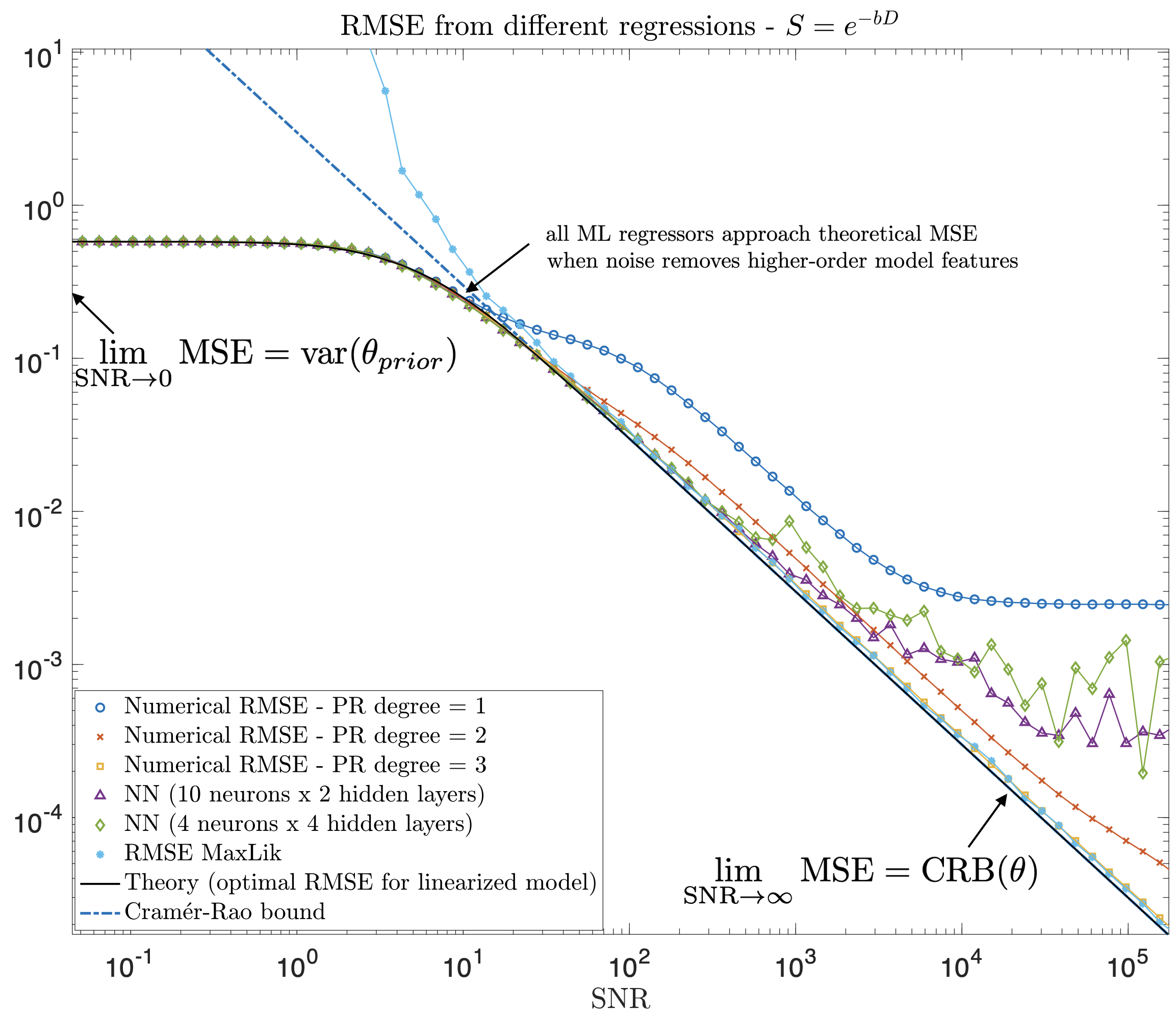
Two regimes. From above, interesting insights can be obtained if we take two limits. For $$$\lim_{x_p\rightarrow\infty}$$$ (high SNR), $$$\mathrm{MSE}_{tr}$$$ tends to the Cramér-Rao bound of $$$\theta$$$, a bound on the lowest achievable variance by an unbiased estimator⁹. Then, taking $$$\lim_{x_p\rightarrow\,0}$$$ (low SNR), we see that $$$\mathrm{MSE}_{tr}$$$ does not increase proportionally to $$$\sigma$$$ but instead reaches a plateau at a value of the variance in the training data. Any regression will at some point behave like the linear, see Fig. 2 for an exponential model.
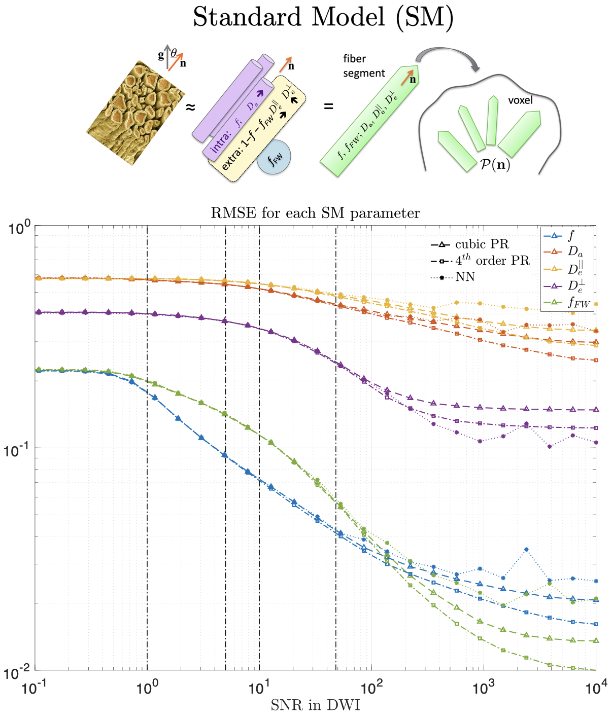
We are usually in-between these two extremes, where data-driven approaches provide lower MSE even if the prior does not match the test distribution. In the case of the Standard Model (SM) of diffusion in white matter¹⁰, a cubic polynomial is usually enough to fit all parameters within a realistic SNR (see Fig. 3 and Experiments for protocol). Since this model is highly nonlinear, a big increase in SNR means more sophisticated regressions will be optimal.

Experiments

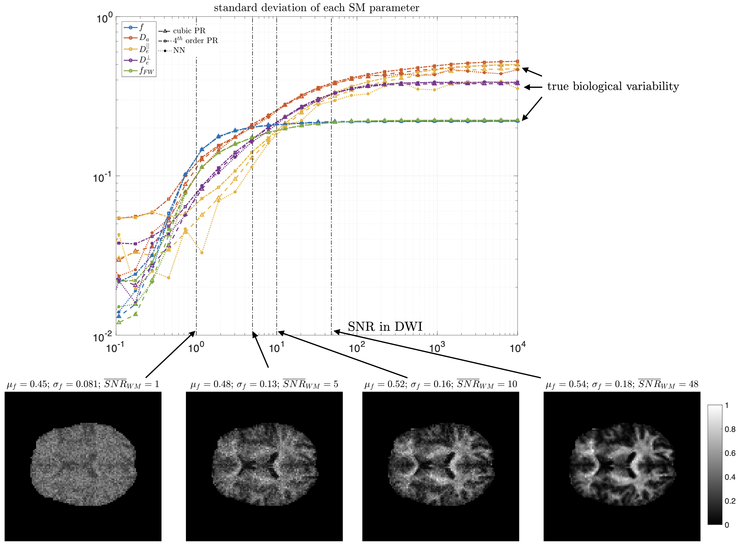
MRI data. A 23yo female volunteer was imaged in a whole-body 3T system (Siemens PRISMA) using a 20-channel head coil. Maxwell-compensated free-gradient diffusion waveforms were acquired¹¹ using a spin echo EPI readout. The protocol had $$$\{6,20,15,40,35,40\}$$$ non-collinear gradient directions at $$$(b,b_\Delta)=[(0,1),(1000,1),(1500,0),(2000,1),(5000,0.8),(5500,1)]\,s/mm^2$$$, totalling 156 DWI. These images were acquired with $$$2\times2\times2\,mm^3$$$ voxels over 72 slices, $$$T_R=5.3s,\,T_E=92ms,\,BW=1600Hz/Px,\,R=2,\,PF=6/8,\,t_\text{acq}=15\,\text{minutes}$$$.

Results. Figure 5 shows histograms of SM estimates for a white matter region of interest (ROI). As we increase the noise in the data, estimates reduce their variance and get shifted towards the mean of the prior. Figure 4 shows that parametric maps that look realistic can be too homogeneous when the SNR is low.

Discussion and Conclusion

For typical noise levels in quantitative MRI the prior distribution may push parameter estimates towards its mean. This is modulated by the SNR, as we showed experimentally and theoretically. At low SNR values, any data-driven regression will behave identically, with their MSE approaching a universal curve independently of the complexity of the regression. Understanding where on this curve is the ML estimation at a given SNR is essential for knowing if we measure tissue parameters, or merely the prior.

Acknowledgements

This work was performed under the rubric of the Center for Advanced Imaging Innovation and Research (CAI2R, https://www.cai2r.net), a NIBIB Biomedical Technology Resource Center (NIH P41-EB017183). This work has been supported by NIH under NINDS award R01 NS088040 and NIBIB awards R01 EB027075.