0361

Combined heating of hip joint implant by radiofrequency and switched-gradient fields during MRI examination

Alessandro Arduino¹, Umberto Zanovello¹, Jeff Hand², Luca Zilberti¹, Rüdiger Brühl³, Mario Chiampi¹, and Oriano Bottauscio¹
¹Istituto Nazionale di Ricerca Metrologica, Torino, Italy, ²School of Biomedical Engineering and Imaging Sciences, King’s College London, London, United Kingdom, ³Physikalisch-Technische Bundesanstalt, Braunschweig and Berlin, Germany

Synopsis

Local heating effects in patients carrying orthopaedic implants have been studied mostly as a consequence of radiofrequency fields and, to a less extent, to gradient coil fields, separately. In this study the heating produced by the combined effects of both fields during realistic clinical sequences is numerically simulated in an anatomical human model carrying a CoCrMo hip implant. Risky situations have been identified, also showing that, sometimes, the gradient field heating can be most significant. The analysis suggests that criteria, based on whole-body SAR only, may not be sufficient to ensure patients’ safety.

INTRODUCTION

Heating effects in patients carrying orthopaedic implants have been studied mostly for RF fields^1-11 and, to a lesser extent, to GC fields^12-20, separately. Concepts for risk assessment and attempts towards active safety management have been discussed in a recently published review article²¹. This work investigates how the simultaneous exposure to GC and RF fields affects the temperature rise in patients with metallic hip prosthesis. The analysis uses realistic clinical sequences and temperature increase within the body, rather than SAR, as a safety metric.

METHODS

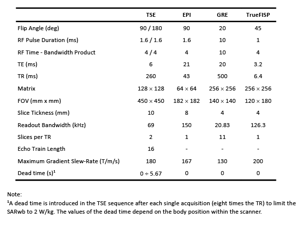
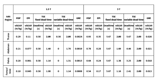
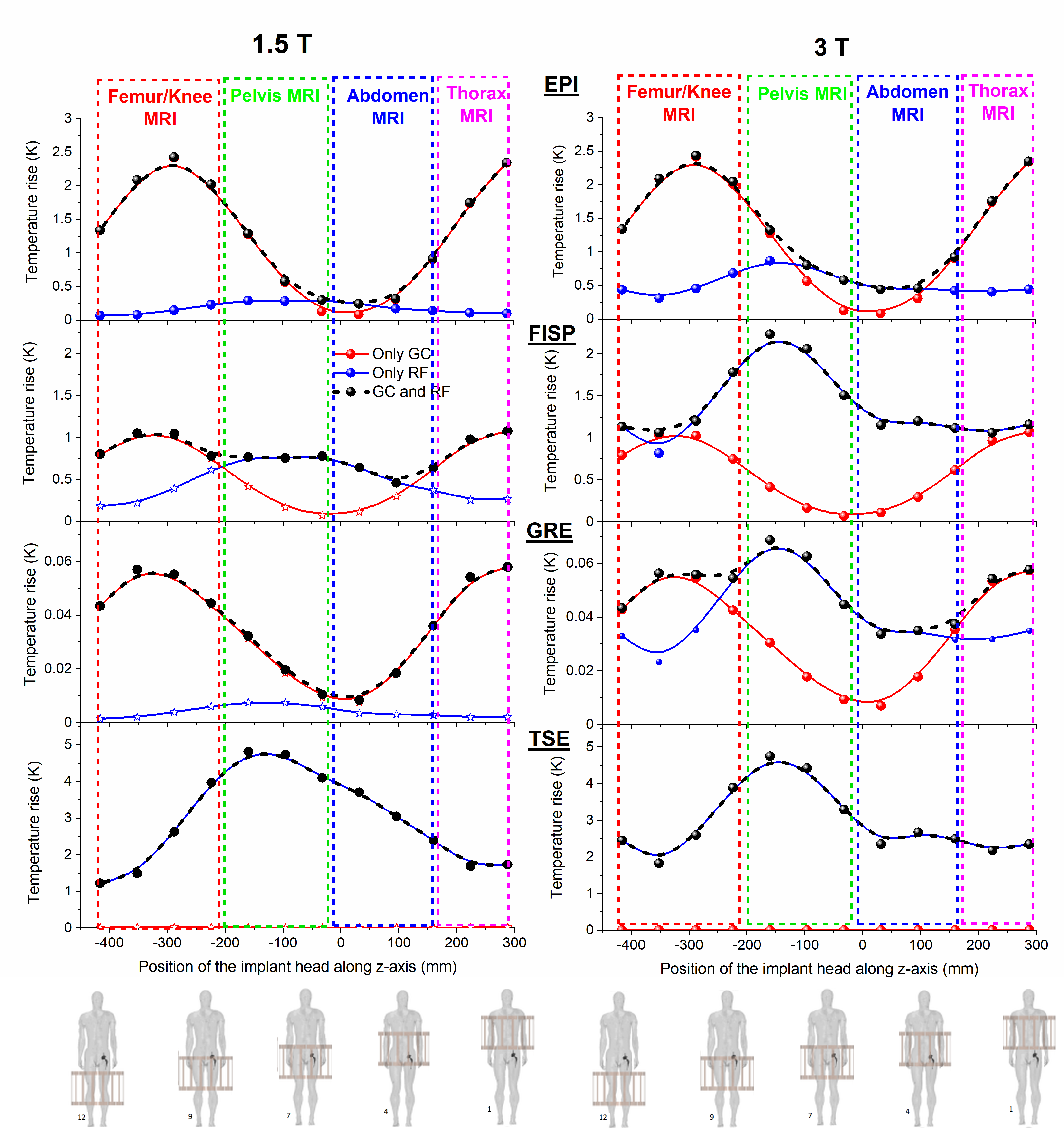
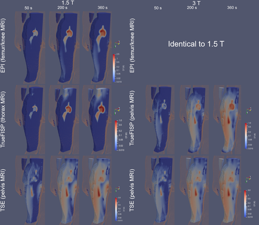
The “Duke” anatomical model²², segmented into 2 mm voxels and modified by inserting an ASTM F75 CoCr alloy hip prosthesis was used. Physical properties of biological tissues were taken from IT'IS database²³. Apart from thermoregulation effects, all properties are independent of temperature. The model of a generic high-pass birdcage, 16-rung, shielded circular RF body coil was provided by an MRI manufacturer. The coil was excited in quadrature and tuned to 123.2 MHz or 63.2 MHz. The model of the GCs represented a realistic set-up used in cylindrical scanners. Turbo spin echo (TSE), EPI, gradient echo (GRE) and TrueFISP sequences were designed with the parameters summarized in Figure 1. Twelve positions of Duke along the scanner’s longitudinal axis associated with different imaging zones, as thorax (pos. 1-2), abdomen (pos. 3-5), pelvis (pos. 6-8), and femur/knee (pos. 9-12), were considered (Figure 3), to investigate the effect of position on implant heating. Whole-body SAR (SARwb) was below 2 W/kg in all cases (Figure 2); for the TSE sequence, a dead time (either variable with position or fixed to that of the worst case) was introduced after each acquisition to guarantee this limit. Thermal simulations were performed as described in a previously published article¹⁹. Computation of RF power deposition was carried out using SEMCAD X v14.8.6²⁴; that associated with the GC fields was calculated as described in a previously published article¹⁹. Results were analyzed in terms of temperature increase after 360 s and 900 s in tissues surrounding the implant. Assuming temperature limits of 39 °C and 41 °C^25-27, thresholds for temperature increase ΔT equal to 1 K and 3 K were considered.

RESULTS

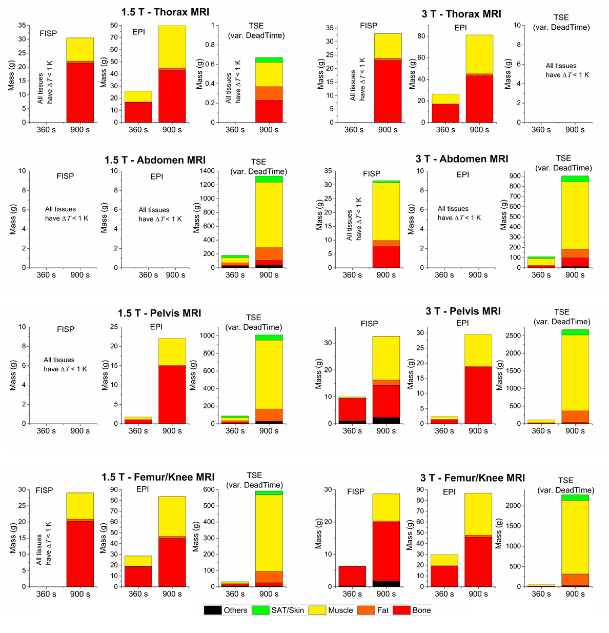
The axial position of the hip implant largely affects heating (Figure 3). The maximum temperatures due to RF and GC are not simply additive due to thermoregulation and the different spatial distributions of ΔT. For GCs, the maximum ΔT occurs for thorax or femur/knee imaging, whereas for RF, highest values are found for pelvis imaging. For TSE the predominant heating is caused by RF, whilst for EPI, GC is the dominant source. The contributions of the two fields are comparable for TrueFISP and GRE. The latter is the least aggressive. Figure 4 shows the thermal evolution around the implant. When GC effects prevail, the voxels exceeding the temperature threshold are mainly close to the implant; this is not always true when the RF field dominates the heating. The mass of tissue within the region of influence and undergoing a ΔT > 1 K was determined after 360 s and 900 s of exposure (Figure 5). The mass with ΔT > 1 K is greater with TSE (up to 2600 g at 3 T and up to 1300 g at 1.5 T after 900 s). With EPI, the greatest heated mass after 900 s is ~85 g, found in thorax and femur/knee MRI. The greatest mass for TrueFISP (~30 g after 900 s) is found for all positions at 3 T. Only the TSE sequence produces ΔT > 3 K, involving 10 ÷ 12 g after 900 s for pelvis and femur/knee MRI, both at 1.5 T and 3 T.

DISCUSSION

RF dominates when the implant is inside the RF coil (e.g. pelvis imaging), in accordance with previously published results⁴. GC heating becomes significant for sequences with higher field changing rate (e.g. EPI) and the implant outside the imaging region (thorax or femur/knee imaging). TSE sequence produced the largest temperature increases, namely ~5.3 K to ~6.1 K for 1.5 T and 3 T, respectively. These results suggest that SARwb does not represent a reliable metric for predicting heating in presence of implants. ΔT thresholds of 1 K and 3 K were exceeded for most sequences. Exceptions were TrueFISP for abdomen and pelvis imaging at 1.5 T and GRE for all positions. For EPI this occurs for femur/knee and thorax imaging and this is representative of any sequence whose heating contribution is dominated by GCs. For TrueFISP the contributions of RF and GC fields are comparable. At 1.5 T, GC heating dominates when imaging thorax and femur/knee, while RF prevails for pelvis and abdomen imaging. At 3 T, the contribution from RF increases and exceeds the GC contributions.

CONCLUSION

This study indicates a need for assessment of GC heating related to implant position and occurrence of maximum change in the gradient fields. Moreover, results emphasize the fact that evaluating potential injury to patient only with standard test methods (e.g. ASTM F2182-19²⁸) does not address all safety concerns.

Acknowledgements

The results here presented have been developed in the framework of the 17IND01 MIMAS Project. This project has received funding from the EMPIR Programme, co-financed by the Participating States and from the European Union’s Horizon 2020 Research and Innovation Programme.

References

1. Nyenhuis JA, Park S-M, Kamondetdacha R, Amjad A, Shellock FG, Rezai AR. MRI and implanted medical devices: Basic interactions with an emphasis on heating. IEEE Trans Device Mater Rel 2005;5:467-480.

2. Murbach M, Zastrow E, Neufeld E, Cabot E, Kainz W, Kuster N. Heating and safety concerns of the radio-frequency field in MRI, Curr Radiol Rep. 2015;3:1-9.

3. Liu Y, Chen J, Shellock FG, Kainz W. Computational and experimental studies of an orthopedic implant: MRI-related heating at 1.5-T/64-MHz and 3-T/128-MHz. J Magn Reson Imaging 2013;37:491-497.

4. Powell J, Papadaki A, Hand J, Hart A, McRobbie D. Numerical simulation of SAR induced around Co-Cr-Mo hip prostheses in situ exposed to RF fields associated with 1.5 and 3 T MRI body coils. Magn Reson Med 2012;68:960–968.

5. Baker KB, Tkach JA, Nyenhuis JA, Phillips M, Shellock FG, Gonzalez-Martinez J, Rezai AR. Evaluation of Specific Absorption Rate as a dosimeter of MRI-related implant heating. J Magn Reson Imaging 2004;20:315-320.

6. Destruel A, O’Brien K, Jin J, Liu F, Barth M, Crozier S. Adaptive SAR mass-averaging framework to improve predictions of local RF heating near a hip implant for parallel transmit at 7 T. Magn Reson Med 2019;81:615-617.

7. Stenschke J, Li D, Thomann M, Schaefers G, Zylka W. A numerical investigation of RF heating effect on implants during MRI compared to experimental measurements. Adv Med Eng 2007;114:53–58.

8. Mohsin SA , Sheikh NM, Abbas W. (2009) MRI induced heating of artificial bone implants. J Electromagn Waves Appl 2009;23:799-808.

9. Muranaka H, Horiguchi T, Ueda Y, Usui S, Tanki N, Nakamura O. Evaluation of RF heating on hip joint implant in phantom during MRI examinations. Jpn J Radiol Technol 2010;66:725–733.

10. Song T, Xu Z, Iacono MI, Angelone LM, Rajan S. Retrospective analysis of RF heating measurements of passive medical implants, Magn Reson Med 2018;80:2726–2730.

11. Yang C-W, Liu L, Wang J et al. Magnetic resonance imaging of artificial lumbar disks: safety and metal artifacts. Chin Med J 2009;122: 911–916.

12. Graf H, Steidle G, Schick F. Heating of metallic implants and instruments induced by gradient switching in a 1.5-Tesla whole-body unit, J Magn Reson Imaging, 2007;26,:1328–1333.

13. Harris CT, Haw DW, Handler WB, Chronik BA. Application and experimental validation of an integral method for simulation of gradient-induced eddy currents on conducting surfaces during magnetic resonance imaging. Phys Med Biol 2013; 58:4367–4379.

14. El Bannan K, Handler W, Chronik B, Salisbury SP. Heating of metallic rods induced by time-varying gradient fields in MRI. J Magn Reson Imaging 2013; 38:411–41.

15. Zilberti L, Bottauscio O, Chiampi M, Hand J, Sanchez Lopez H, Bruhl R, Crozier S. Numerical prediction of temperature elevation induced around metallic hip prostheses by traditional, split, and uniplanar gradient coils. Magn Reson Med 2015;74:272–279.

16. Zilberti L, Arduino A, Bottauscio O, Chiampi M. The underestimated role of gradient coils in MRI safety. Magn Reson Med 2017;77:13–15.

17. Stroud J, Stupic K, Walsh T, Celinski Z, Hankiewicz JH. Local heating of metallic objects from switching magnetic gradients in MRI. Proc SPIE 10954 Medical Imaging, 2019, San Diego, California, United States. doi: 10.1117/12.2512903.

18. Brühl R, Ihlenfeld A, Ittermann B. Gradient heating of bulk metallic implants can be a safety concern in MRI. Magn Reson Med 2017;77:1739–1740.

19. Arduino A, Bottauscio O, Brühl R, Chiampi M, Zilberti L. In silico evaluation of the thermal stress induced by MRI switched gradient fields in patients with metallic hip implant. Phys Med Biol 2019;64:245006. doi: 10.1088/1361-6560/ab5428.

20. Liu F, Zhao H, Crozier S. On the induced electric field gradients in the human body for magnetic stimulation by gradient coils in MRI. IEEE Trans Biomed Eng 2003;50:804-815. doi: 10.1109/TBME.2003.813538.

21. Winter L, Seifert F, Zilberti L, Murbach M, Ittermann B. MRI-related heating of implants and devices: A Review. J Magn Reson Imaging 2020; Early View, https://doi.org/10.1002/jmri.27194.

22. Sim4Life, Computable human phantoms, Zurich MedTech AG, Zurich, https://zmt.swiss/sim4life/

23. Hasgall PA, Di Gennaro F, Baumgartner C, Neufeld E, Lloyd B, Gosselin MC, Payne D, Klingenböck A, Kuster N. IT’IS Database for thermal and electromagnetic parameters of biological tissues, Version 4.0, May 15, 2018, DOI: 10.13099/VIP21000-04-0. Itis.swiss/database.

24. SEMCAD v14.8.6, Schmid & Partner Engineering AG, Zurich, Switzerland

25. International Electrotechnical Commission (IEC) IEC 60601-2-33:2010 +AMD1:2013+AMD2:2015: Medical electrical equipment - particular requirements for the basic safety and essential performance of magnetic resonance equipment for medical diagnosis, Edition 3.2. IEC, Geneva, 2015.

26. ICNIRP guidelines for limiting exposure to electromagnetic fields (100 kHz TO 300 GHz). Health Phys 2020;118:483–524.

27. ICNIRP statement Medical Magnetic Resonance (MR) procedures: protection of patients. Health Phys 2004;87:197–216.

28. F2182-19 Standard test method for measurement of Radio Frequency induced heating on or near passive implants during magnetic resonance imaging. ASTM International, 2019.

Figures

Figure 1: List of main parameters associated with the four analysed sequences. An apodization factor equal to 0.5 has been used for all the sinc shaped RF pulses.

Figure 2 –SARwb (W/kg) for the imaging regions (body/coil positions) and sequences. For the TSE sequence, a dead time either fixed or variable with position (up to 0.30 s for 1.5 T and up to 5.67 s for 3 T) was adopted to keep SARwb below 2 W/kg.

Figure 3 – Maximum temperature increase in the whole body volume after 360 s exposure versus the axial position of the hip implant in the coils, corresponding to the twelve body positions from 1 to 12. Results for EPI, True-FISP, GRE and TSE (with constant dead time) sequences. Dimensions of the prosthesis: stem length 142 mm; hemispherical head diameter 30 mm; acetabular shell diameter and thickness 66 mm and 8 mm; screw length 34 mm; polyethylene liner thickness 10 mm.

Figure 4 – Time-spatial evolution of the temperature increase around the prosthesis for three analysed sequences (screenshots after 50 s, 200 s and 360 s). For the 3 T group, the results for the EPI sequence are not reported, being almost identical to those at 1.5 T. The results for the TSE sequence refer to a constant dead time of 5.67 s. A region of influence around the implant was defined as a parallelepiped box of size 21.7 cm × 18.8 cm × 28.2 cm.

Figure 5 – Mass of most significant tissues around the implant which exhibit a temperature increase ΔT (after 360 s and after 900 s) greater that the threshold of 1 K. For the TSE sequence, the masses computed with variable dead times for all positions are reported. Within each bar, the colour indicates the fraction associated to a given tissue.

Proc. Intl. Soc. Mag. Reson. Med. 29 (2021)

0361