Introduction

The non-linear mathematical relationship between the MRI signal and the biophysical contrast sources has been a significant challenge of quantitative MRI (qMRI). While Deep Learning (DL) has recently achieved unprecedented performance in solving non-linear problems of various kinds¹, network training often relies on extensive ground-truth training data. Such training data is often not available in qMRI, primarily when novel techniques aim to quantify properties that have been inaccessible before.

The present work illustrates how a fully unsupervised physics-informed DL algorithm can solve such problems with data from as low as N=1 subject. As a proof-of-concept application, we implemented a network that quantifies R₂*, B₀, and the transceiver phase from complex-valued bipolar multi-echo gradient-recalled echo (GRE) data. Established state-of-the-art algorithms for this task are computationally expensive and unstable multi-step procedures.^2,3

Methods

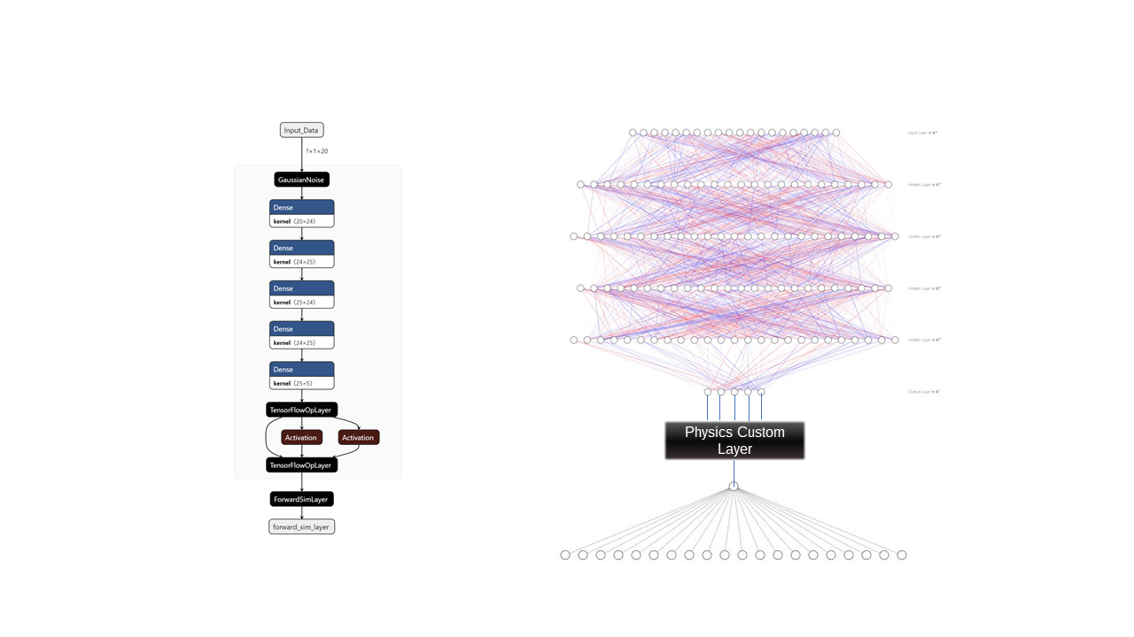
Neural Network Architecture: We implemented a custom deep neural network (Tensorflow 2; Fig. 1) with an encoder (inversion) and a decoder (forward-simulation) part. The number of nodes in the input and output layers was equal. We added two input nodes (real and imaginary) for each of the M GRE-echoes, resulting in 2M input/output nodes. The loss function was the mean squared difference between the measured MRI signal (input) and the network prediction, ensuring data fidelity and an appropriate (Gaussian) noise model. We included one node for each tissue quantity to be determined in the layer that separated encoder and decoder parts. To enforce the physical relevance of these quantities, we used the following MR-physics model in the decoder part:

$$S(\mathrm{TE}) = A_{0}\cdot e^{-\mathrm{TE}\cdot R^{*}_{2} + i[\omega\cdot \mathrm{TE} + \omega_{\mathrm{TE} = 0} + \Delta\omega_{gr}(\mathrm{TE})]} \:(\mathrm{Equation\:1})$$

with TE being echo time, ω frequency, ω_{TE = 0} transceiver phase, and Δω_gr(TE) the gradient-polarity-related phase difference. Positivity of quantities, if appropriate, was enforced through activation function choice. We used a fully connected network with three hidden layers in the decoder part. A Gaussian noise layer was added after the input layer to improve conditioning.

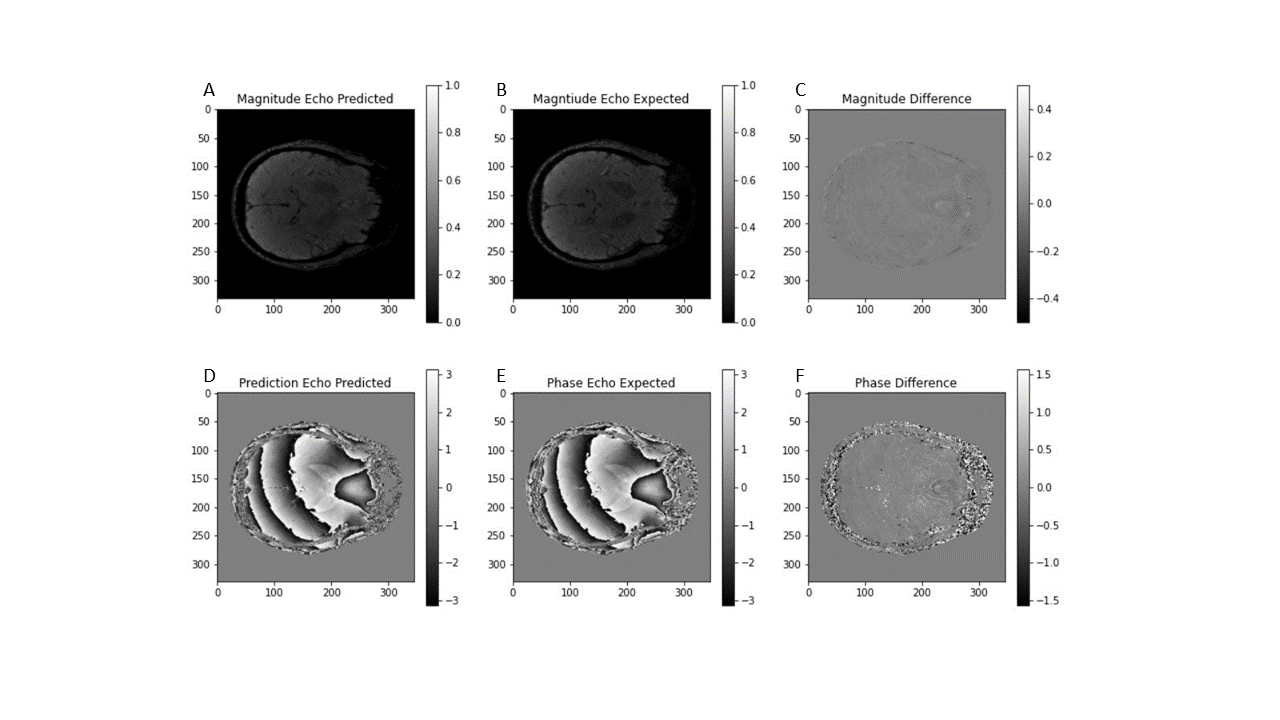
Network Training: We trained the network on single-voxel volunteer GRE data (N=1) acquired with a 6.5 minutes axial whole-brain 3D multi-echo GRE sequence at 3T (TR/TE₁/ΔTE=30.4/4/2.5 ms; 10 echoes, flip 14°; 558 Hz/px; 0.67x0.9x1.8 mm³; Fig. 2b,e). We used ADAM⁴ optimization on one GPU (NVIDIA GeForce RTX 2080 Ti).

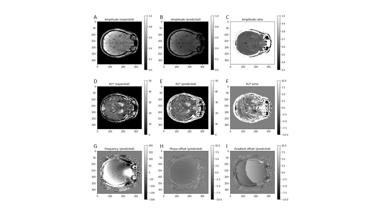
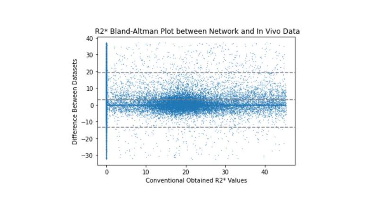
Evaluation: We extracted the tissue quantities (Figure 3) from the separation layer and compared them to parameters obtained with conventional least-squares fitting of denoised magnitude data (Figures 3 and 4).

Results

The training loss converged after 2500 epochs, and training was stopped after 2 hours at 7000 epochs. Figure 2a,d shows the predicted (output) magnitude and phase images of the 10-th echo, which was highly similar to the input (Fig. 2c,f), illustrating that the parameters at the separation layer appropriately describe the measured signal throughout the brain. Figure 3a-f contrasts the predicted tissue parameters with those obtained by conventional methods. The resulting field map (Fig. 3g) was free of wraps and showed typical tissue contrast, the transceiver phase (Fig. 3h) demonstrated typical non-harmonic behavior, and the gradient-polarity-related phase showed a linear spatial pattern (Fig. 3i), as expected. Relaxation rate and A₀ were similar to those obtained with conventional methods. Figure 4 quantifies the prediction errors of the parameter maps compared to those obtained with conventional methods. Computation time for whole-brain prediction from complex-valued data was 6.5 seconds.

Discussion

This study demonstrated the feasibility of solving inverse problems of qMRI with DL entirely based on the theoretical signal model and measured MRI signals. Theoretical models are usually available and can be more complicated than the one used here. Ground-truth training data (labels) are not needed. The implemented network yielded maps in a single computational pass whose computations require multiple, independent processing steps with established techniques, some of them ill-conditioned. Since the proposed network works on raw data, it correctly accounts for the signal noise, different from most magnitude-based processing algorithms. Results were similar to the conventional methods but not identical. However, it remains unclear if the predicted R₂* or the conventional R₂* is more correct because model inaccuracies in established methods render them a questionable gold standard. Since the implemented network yielded accurate frequency and phase maps throughout the brain without wrapping artifacts, despite its voxel-by-voxel nature, it may perform well with phase data that can be difficult to unwrap, such as in the presence of spatial discontinuities.

Conclusion and Outlook

Network training without ground truth data allows inverting complex theoretical signal models that could not be inverted until recently due to inefficient numerical techniques. Future research will validate the proposed framework systematically, evaluate generalization, and investigate the incorporation of more advanced biophysical multi-compartment models in the decoder part of the network and additional MR measurements in the input layer. The proposed neural network framework may allow fast and comprehensive tissue characterization in qMRI with complex signal models that have been difficult to solve with conventional techniques.

Acknowledgements

This study was supported by an equipment grant from Canon Medical Systems Corporation and Canon Medical Research USA, Inc. Research reported in this publication was funded by the National Center for Advancing Translational Sciences of the National Institutes of Health under Award Number UL1TR001412. The content is solely the responsibility of the authors and does not necessarily represent the official views of the NIH.