Introduction

Fast and accurate modeling of MR signal responses are typically required for quantitative MRI applications, such as MR Fingerprinting (MRF)¹ and MR-STAT². Taking MR Fingerprinting dictionary generation as an example, the computational time for simulating large amount of MR signals can be prohibitively long, from hours to days, especially when slice profile effects are taken into account³.
Based on recent development in deep learning, we propose a Recurrent Neural Network (RNN) architecture with multiple stacked layers for quickly computing large-scale MR signals and derivatives for transient-state gradient-spoiled sequences. Two main advantages of the RNN model are its generalization capability and computational efficiency: the same RNN model works with different sequence parameters, such as sequence length and time-dependent flip-angle train without need for retraining. We show that the RNN surrogate model can be used for orders of magnitude acceleration of different qMRI applications, in particular MRF dictionary generation and optimal experimental design.

Methods

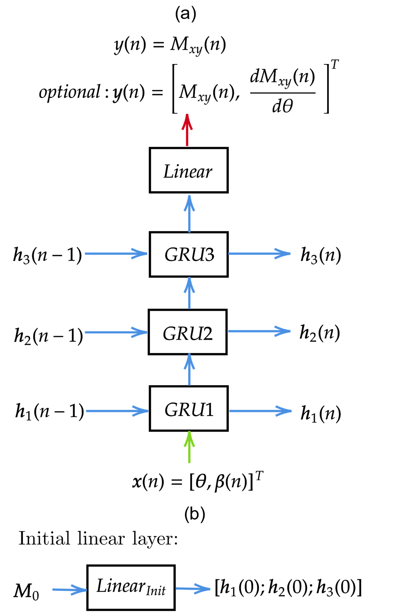
• Network architecture

RNN models can be effectively used to model time-dependent processes and especially ordinary differential equations, therefore they are very suitable for MR signal computations. Specifically, an RNN architecture with three stacked Gated Recurrent Units (GRU)⁴ is selected (Fig.1). Fig.1(a) shows the RNN structure for the $$$n$$$-th time step, which includes three GRU layers and one Linear layer. The inputs for the $$$n$$$-th RF pulse are tissue specific parameters $$$\mathbf{θ}=[T_1,T_2]^T$$$ and time-dependent sequence parameters $$$\mathbf{β}(n)=[T_R(n), T_E(n),\alpha(n)]^T$$$, where $$$\alpha(n)$$$ is the RF flip-angle. The final linear layer generates the transverse magnetization signal $$$M_{xy}(n)$$$ and derivative signal $$$dM_{xy}(n)/d\mathbf{θ}$$$. The whole network has only 16643 trainable parameters.

• Data generation and network training

A dataset containing 30000 magnetization signals was simulated from an EPG model⁵ which included the finite RF pulse duration effects. Each EPG signal was simulated using a gradient-spoiled sequence with 1120 Gaussian-shaped RF pulses. Randomly selected tissue parameters ($$$T_1\in [0.1,5]$$$s and $$$T_2\in [0.01,2]$$$s) and sequence parameters ($$$T_R(n)\in [5,20]$$$ms and $$$T_E(n)\in [0.3T_R(n),0.7T_R(n)]$$$ms) were used. Four different types of flip-angle trains, $$$\mathbf{\alpha}=[\alpha(1),\alpha(2),...\alpha(n)]^T$$$, were also used for dataset generation, as shown in Fig.2(a).
The dataset was split into a training set of size 20000 and a test set of size 10000. The RNN network was built and trained using Tensorflow 2.2 on a Tesla-V100-GPU, run for 3000 epochs, ADAM optimizer using Mean Absolute Error loss function, batch size 200.

• Applications

Two examples of qMRI applications are presented. The first one is accelerated MRF dictionary generation. A gradient-spoiled transient-state sequence with single-spoke radial acquisition was used⁶. In-vivo brain data was collected on a Philips Ingenia 3T scanner, and was reconstructed⁷ using either the RNN generated or the conventional EPG generated dictionary.
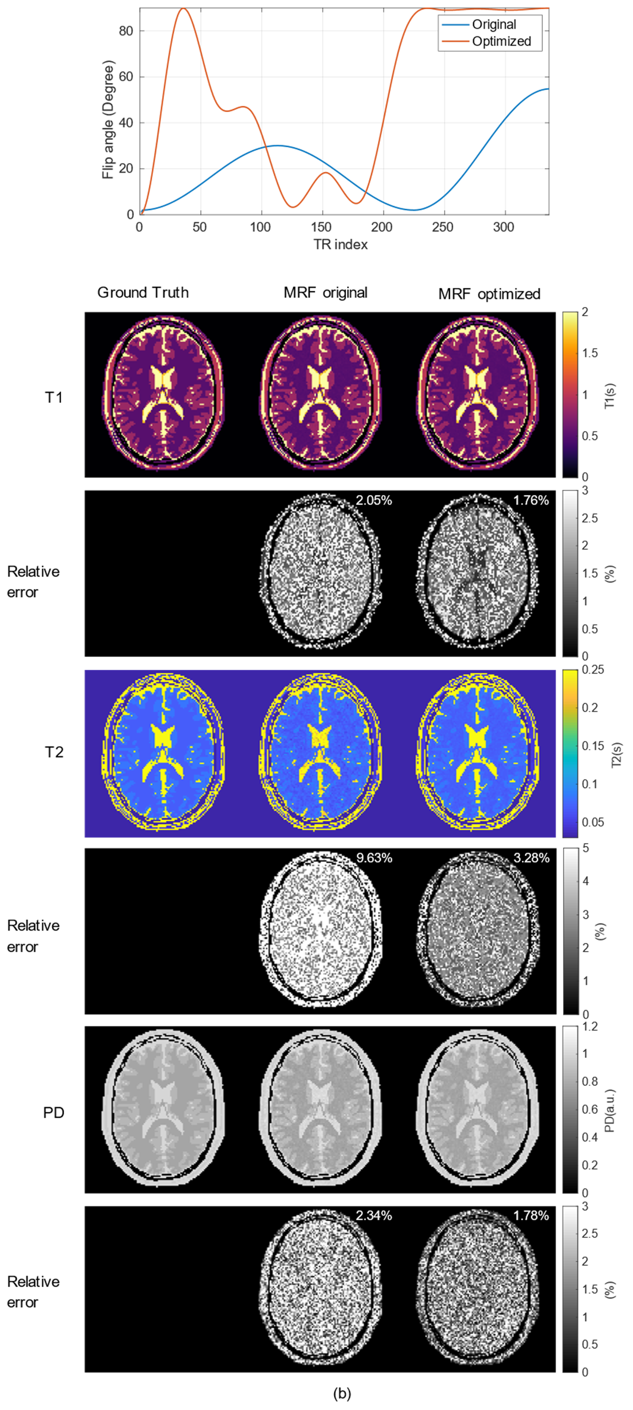
The second example is MRF sequence optimization. Specifically, the problem is to find the optimal flip-angle train for minimizing the reconstruction noise which is characterized by the Cramér-Rao lower bound (CRLB)⁸. We conducted a simulation-based experiment to optimize a Spline11-type flip-angle train given two target tissues with $$$T_1/T_2=900/85$$$ms and $$$T_1/T_2=500/65$$$ms. The sequence length is 336 with $$$T_E/T_R=4.9/8.7$$$ms. Constrained differential evolution was used for solving the optimization problem, and the RNN model was used for accelerating the CLRB computation.

Results

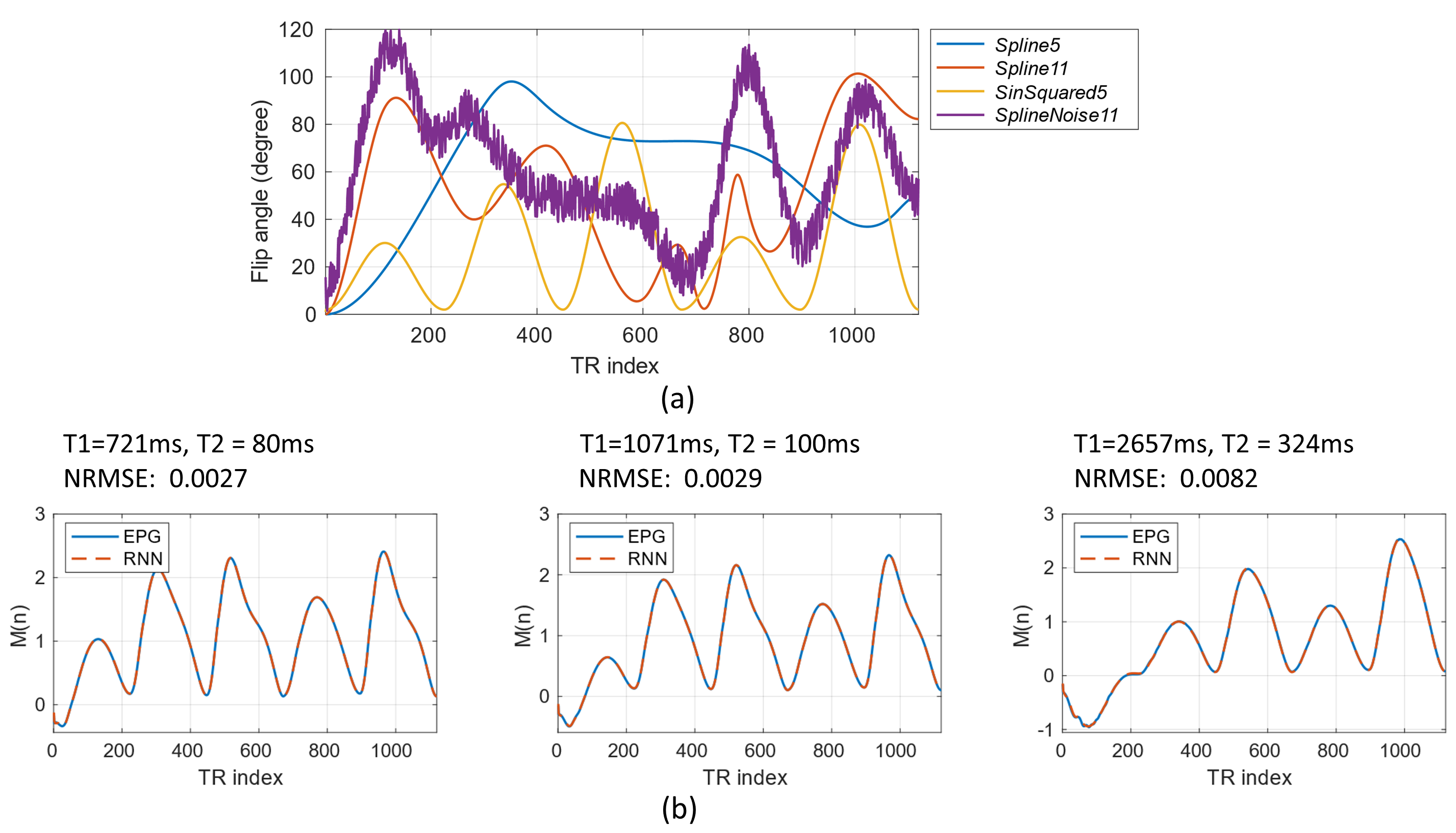
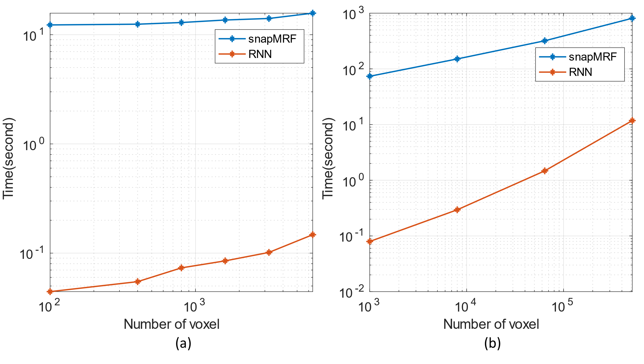
The total training took approximately 8 hours. Fig.2(b) shows sample RNN signals are in excellent agreement with EPG signals. The overall NRMSEs for test dataset are relatively low: 0.77% for magnetization signals and 1.39% for signal derivatives, showing that the proposed RNN is able to accurately model the signal even for unseen flip angle trains.
Fig.3 shows the runtime comparison results for our RNN and the recently proposed fast GPU simulator snapMRF⁹. In Fig.3(a) and 3(b), all the runtime curves grow approximately linearly with respect to the number of signals. For the fixed $$$B_1^+$$$ condition in Fig.3(a), RNN requires ~100 times shorter runtime than snapMRF for a dataset with 6400 signals. For various $$$B_1^+$$$ conditions (a large dataset with 512000 signals) , our RNN outperforms snapMRF by a factor of 68 (Fig.3(b)).
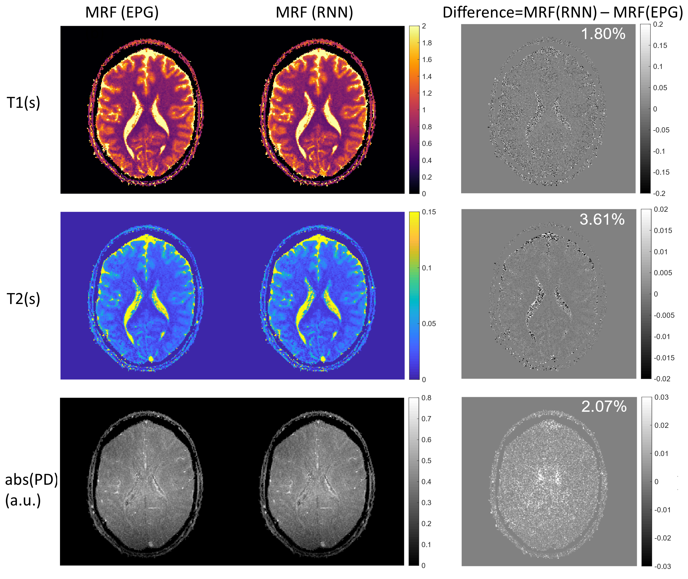
Fig.4 shows that in-vivo MRF reconstructions using EPG or RNN generated dictionaries are very similar. Generating the dictionary with 7812 signals by RNN takes just 0.3s, whereas running the EPG model on CPU takes about 1.7 hours.
Fig.5(a) shows the optimized flip-angle train and Fig.5(b) shows the MRF-reconstructed $$$T_1, T_2$$$ and $$$abs(PD)$$$ maps using the original and optimized sequences. The optimized sequence improves the accuracy of all the three reconstructed maps comparing to the original sequence, with a most significant improvement in $$$T_2$$$ maps. Solving the sequence optimization problem now takes about 10.5 seconds, whereas in previous works¹⁰, solving similar problems requires at least one CPU hour.

Discussion and Conclusion

This work proposed a RNN model as a fast surrogate of the EPG model for computing large-scale MR signals and derivatives. We demonstrated that the RNN model is between one and three orders of magnitude faster than the GPU-accelerated EPG package snapMRF⁹. The RNN surrogate model can be efficiently used for computing large-scale MRF dictionary signals and derivatives within seconds. The practical application of transient-state quantitative techniques can therefore be substantially facilitated. In the future, usage of the RNN model may be extended for other types of sequences, or for modeling more complex physics such as magnetic transfer effects. Code is freely available at https://gitlab.com/HannaLiu/rnn_epg.

Acknowledgements

The first author receives CSC(Chinese Scholarship Counsel) scholarship.