0328
DeepTSE-T2: Deep learning-powered T2 mapping with B1+ estimation using a product double-echo Turbo Spin Echo sequence1Department of Electrical and Computer Engineering, Seoul National University, Seoul, Korea, Republic of, 2Department of Radiology, Seoul St Mary’s Hospital, College of Medicine, The Catholic University of Korea, Seoul, Korea, Republic of, 3Siemens healthineers Ltd, Seoul, Korea, Republic of, 4Division of Biomedical Engineering, Hankuk University of Foreign Studies, Yongin, Korea, Republic of
Synopsis
We developed DeepTSE-T2, a deep learning-based T2 mapping algorithm with retrospective B1+ estimation for a product double-echo TSE sequence. DeepTSE-T2 enables T2 mapping by retrospectively estimating B1+ information, reconstructing T2 in high-accuracy (NRMSE = 8.26 ± 0.30%). The proposed method is useful in a clinical setting since it utilizes a fast imaging product sequence. The training dataset consists of simulation-based data, providing flexibility in parameter setting. Applications to χ-separation and an MS patient are included.
Introduction
Quantification of T2 has been suggested to provide valuable information of tissues.1,2 However, T2 mapping via a multi-echo spin-echo (MESE) sequence requires a long scan time, and suffers from a high specific absorption rate. To overcome such limitations, various fast T2 mapping methods were introduced.3,4 However, these methods require sequence modification and are not available widely. Recently, double-echo TSE (DE-TSE)-based T2 mapping was developed using additional B1+ map acquisition.5 This approach has advantages of using a product sequence and the PDw and T2w images can be used for clinical diagnosis. Furthermore, the scan time is short acquiring 30 slices in 2 min (for comparison, MESE: 11 min). However, the method requires an additional B1+ scan, costing time (+2 min). In this study, we propose a deep learning-based T2 mapping algorithm for DE-TSE. A B1+ map was estimated from the DE-TSE images using a neural network (i.e. no additional scan). Then the B1+ information along with DE-TSE images is utilized for a deep neural network reconstruction of a T2 map. The results are utilized for quantitative analysis of an MS patient and χ-separation6 for susceptibility imaging.Methods
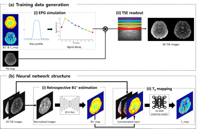
[Training data] Training DE-TSE data are generated using the maps from MESE data of 11 subjects,7 (training: 10, validation:1) utilizing EPGSLR7 and TSE readout scheme (Fig. 1a). The training data consist of 2280 slices.[DeepTSE-T2] DeepTSE-T2 is composed of two steps. In the first step, a 2D U-net8 is used to estimate the B1+ map from the second echo TSE image normalized by the first echo image. Then, the B1+ map and DE-TSE images are concatenated as an input for a voxel-based artificial neural network (ANN), estimating T2 values (Fig. 1b). The loss function is the sum of the model loss and L1 loss between output and label. The model loss is implemented using a pre-trained 2D U-net trained to estimate the forward model of B1+ and T2 maps to a DE-TSE image.
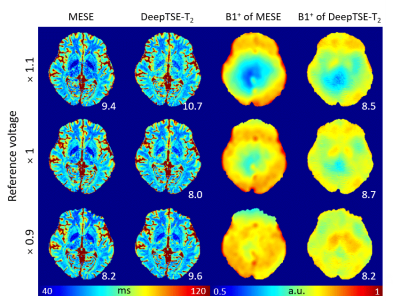
[Evaluation] Six healthy subjects are utilized to evaluate the performance of DeepTSE-T2. For the quantitative evaluation, retrospective DE-TSE images are generated from the 2D MESE data and prospective DE-TSE images are acquired (all data IRB-approved). DeepTSE-T2 results are compared to those of an end-to-end U-net as well as a few EPGSLR-based fitting methods with extra B1+ information. Normalized root-mean-squared error (NRMSE), peak signal to noise ratio (PSNR), and structural similarity (SSIM) between the reconstructed image and label (T2 map from MESE7) are calculated with CSF masked out. To demonstrate robustness to B1+ variations, three data are acquired with different reference voltages and evaluated.
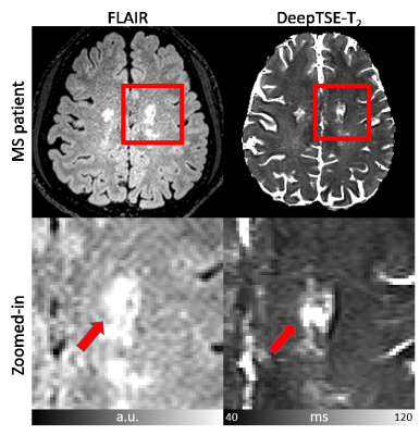
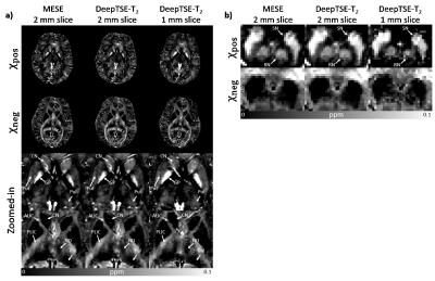
[Applications] Two T2 maps (1 mm and 2 mm slice thickness) reconstructed with DeepTSE-T2 are applied to the χ-separation algorithm6. The results are compared to those with T2 from MESE. Additionally, an MS patient data are utilized to assess generalization to unseen data distribution.
[Datasets] (Training and validation) MESE data in reference6 was used. (Evaluation) MESE (TR/TE=6200/9:9:90 ms, and TA=11:17), DE-TSE (TR/TE=6200/9,90 ms, ETL=5, and TA=2:24) were acquired (common parameter: FOV=192×192 mm2, voxel size=1×1 mm2, GRAPPA=2, 30 slices, and slice thickness=2 mm). B1+ map was also acquired.9 (χ-separation) MESE (TR/TE=5060/9:9:90 ms, 40 slices, and TA=9:33), DE-TSE2mm (TR/TE=8000/9,90 ms, 40 slices, and TA=3:06), DE-TSE1mm (TR/TE=10000/10.6/106 ms, average=2, 80 slices, and TA=2×3:52) were acquired (common parameter: FOV=192×192 mm2, voxel size=1×1 mm2, GRAPPA=2). 3D GRE was also acquired. (MS patient) One MS patient (43-year-old male) were scanned. FLAIR and DE-TSE (FOV=209×209mm2, voxel size=0.69×0.69 mm2, TR/TE=11000/10,100 ms, ETL=7, FA=150°, slice thickness=2 mm, and TA=5:41) were acquired.
Results
Figure 2 compares the T2 and B1+ maps from DeepTSE-T2 and EPGSLR fitting methods. The DeepTSE-T2 maps provide a high-quality T2 map, comparable to EPGSLR fitting with B1+ from MESE (NRMSE: 8.26 ± 0.30% in DeepTSE-T2; 7.80 ± 0.61% in EPGSLR fitting). Compared to the U-net, DeepTSE-T2 shows lower NRMSE values in both T2 and B1+ estimations (T2: 8.26 ± 0.30% in DeepTSE-T2 and 11.2 ± 1.48% in U-net; B1+: 5.99 ± 0.98% in DeepTSE-T2 and 7.70 ± 1.69% in U-net). Moreover, DeepTSE-T2 results show consistency even at different B1+ reference voltages, showing the robustness to B1+ variations (Fig. 3; NRMSE errors similar between the two methods). Figure 4 shows the FLAIR image and T2 map obtained in the MS patient. As indicated by the red arrows, DeepTSE-T2 can reconstruct T2 values in MS lesions. Figure 5 shows the results of applying the DeepTSE-T2 map to χ-separation. For 2 mm slice thickness, both positive and negative susceptibility maps show similar contrasts to the MESE results. DeepTSE-T2 enables χ-separation in 1 mm slice thickness in a reasonable scan time (DE-TSE: 7:44 min).Conclusion and Discussion
In this study, we developed DeepTSE-T2, a T2 mapping algorithm based on deep learning, for a double-echo TSE product sequence. Compared to the conventional fast T2 mapping method, the method does not require any sequence modification and fast in data processing (4 sec for whole brain).Acknowledgements
This work was supported by the National Research Foundation of Korea (NRF) grant funded by the Korea government(MSIT) (No. NRF-2018R1A2B3008445, NRF-2017M3C7A1047864).References
1. Dunn, T. C., Lu, Y., Jin, H., Ries, M. D., & Majumdar, S. (2004). T2 relaxation time of cartilage at MR imaging: comparison with severity of knee osteoarthritis. Radiology, 232(2), 592-598.
2. Giri, S., Chung, Y. C., Merchant, A., Mihai, G., Rajagopalan, S., Raman, S. V., & Simonetti, O. P. (2009). T2 quantification for improved detection of myocardial edema. Journal of cardiovascular magnetic resonance, 11(1), 56.
3. Deoni, S. C., Peters, T. M., & Rutt, B. K. (2005). High‐resolution T1 and T2 mapping of the brain in a clinically acceptable time with DESPOT1 and DESPOT2. Magnetic Resonance in Medicine, 53(1), 237-241.
4. Warntjes, J. B. M., Leinhard, O. D., West, J., & Lundberg, P. (2008). Rapid magnetic resonance quantification on the brain: optimization for clinical usage. Magnetic Resonance in Medicine, 60(2), 320-329.
5. McPhee, K. C., & Wilman, A. H. (2015). T2 quantification from only proton density and T2-weighted MRI by modelling actual refocusing angles. NeuroImage, 118, 642-650.
6. Shin, H. G., Lee, J., Yun, Y. H., Yoo, S. H., Jang, J., Oh, S. H., ... & Kim, W. (2020). In-vivo histology of iron and myelin in the brain using magnetic susceptibility source separation in MRI. bioRxiv.
7. Lebel, R. M., & Wilman, A. H. (2010). Transverse relaxometry with stimulated echo compensation. Magnetic resonance in medicine, 64(4), 1005-1014.
8. Ronneberger, O., Fischer, P., & Brox, T. (2015, October). U-net: Convolutional networks for biomedical image segmentation. In International Conference on Medical image computing and computer-assisted intervention (pp. 234-241). Springer, Cham.
9. Jiru, F., & Klose, U. (2006). Fast 3D radiofrequency field mapping using echo‐planar imaging. Magnetic Resonance in Medicine, 56(6), 1375-1379.
Figures


