0303
Background Phase Error Reduction in Phase-Contrast MRI based on Acoustic Noise Recordings1Institute for Biomedical Engineering, University and ETH Zurich, Zurich, Switzerland
Synopsis
This work identifies mechanical resonances of the gradient coil system as a source of increased spatially linear and quadratic phase offsets. Mechanical resonance frequencies were identified by mobile phone audio recordings from inside the scanner room and compared to the gradient modulation transfer function. Results demonstrate that optimal TE reduces phase ramps by a factor of 15 and optimal TR removes the spatially quadratic phase offset.
Introduction
Velocity biases in phase-contrast (PC) velocity mapping, such as 4D flow MRI, can compromise accuracy and reproducibility1. These offsets stem from phase differences between the flow encoded and reference segment and are due to unwanted, non-flow sources. Giese et al.2 demonstrated that the phase offset is influenced by mechanical resonances of the gradient system. Despite the availability of valuable approaches for background phase error correction and sequence optimization3, clinical acceptance with a maximum phase offset of 0.4% of venc1 may only be achieved when applying higher order corrections4. In this work we demonstrate background phase error reduction by acoustic noise-guided adjustment of the echo and repetition time of PC sequences.Theory
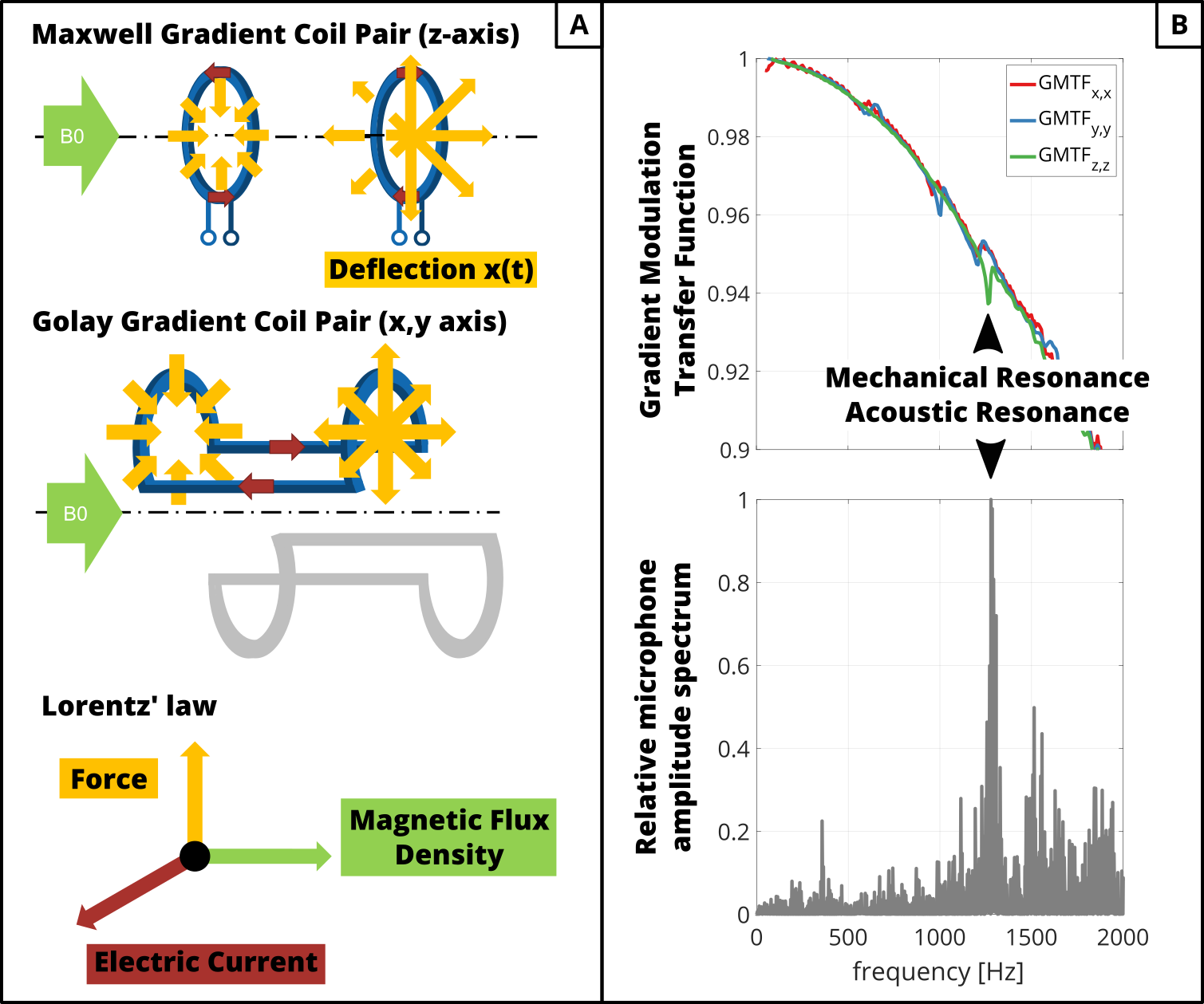
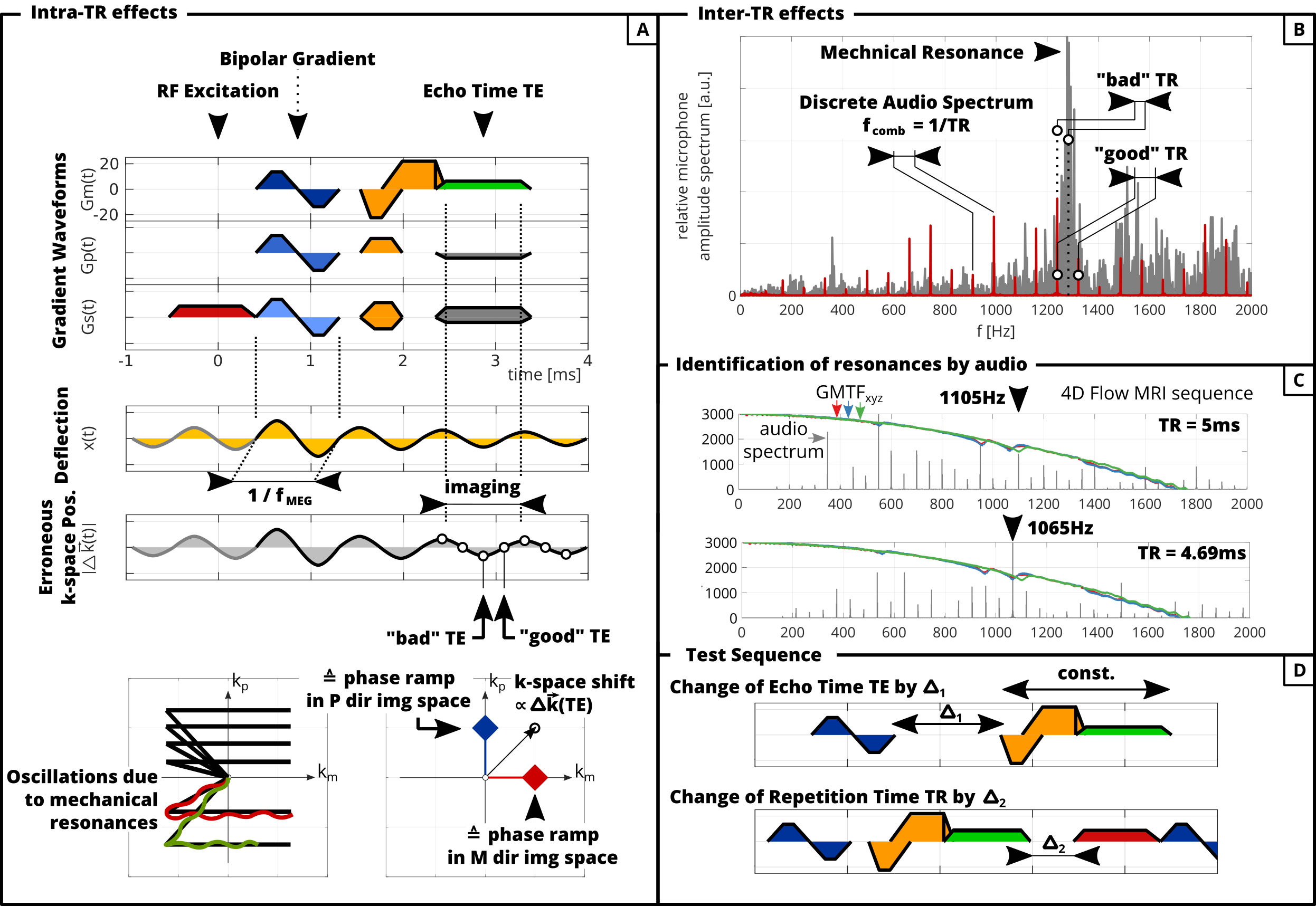
Switching of electric currents leads to Lorentz forces acting on the gradient coils (Figure1A). The deflection results in a change of the magnetic field gradient, which is identified as a peak in the Gradient Modulation Transfer Function (GMTF). The mechanical resonance causes the gradient system to vibrate, which results in acoustic noise (Figure1B). This enables the identification of mechanical resonances by acoustic noise measurements.Changes in the magnetic field gradient lead to an erroneous k-space position$$$\;\Delta{}\vec{k}(t)\;$$$(Figure2A). In phase-contrast images,$$$\;\Delta{}\vec{k}(t)\;$$$is given by the changes in gradient waveforms between encoded and reference segments (bipolar gradient). Depending on$$$\;\Delta{}\vec{k}(\mathrm{TE})\;$$$at echo time$$$\;\mathrm{TE}$$$, the k-space center is shifted resulting in phase ramps in the direction of flow encodings. We term this error “intra-TR effects” and distinguish between “good” $$$\;\mathrm{TEs}\;$$$($$$\Delta \vec{k}(TE)=0$$$) or “bad”$$$\;\mathrm{TEs}\;$$$($$$\Delta\vec{k}(TE)$$$=max), with small or large phase ramps in image space, accordingly. If the inverse of the bipolar gradient duration coincides with a mechanical resonance frequency ($$$f_{res}$$$, Figure2A,C), it is likely that the resonance is excited.
Due to the repetitive nature of MR sequences, the gradient waveform spectrum and the audio spectrum are inherently multiplied by frequency comb$$$\;f_{comb}=1/\mathrm{TR}\;$$$($$$\;\mathrm{TR}\;$$$: repetition time; Figure2B). If comb maxima coincide with peaks of the mechanical resonance spectrum, constructive interference occurs and all axes can be influenced. We term this behavior “inter-TR effects”. Depending on the resonance frequency$$$\;f_{res}\;$$$, we can distinguish between “bad”$$$\;\mathrm{TRs}\;$$$(overlap of$$$\;f_{res}\;$$$and$$$\;f_{comb}$$$) and “good”$$$\;\mathrm{TRs}\;$$$(no overlap).
Methods
A gradient-echo sequence5 (Figure2A,D) was adapted to include bipolar motion encoding gradients (MEG) of frequency$$$\;f_{MEG}\;$$$to acquire sagittal, non-oblique 3D PC MRI images with referenced flow encoding. A static phantom (TX/water,1:12 doped with 0.16ml/l Gadolinium,T1~1s) was scanned on a 3T system (Ingenia; Philips Healthcare, Best, the Netherlands) and offset from the isocenter (32mm in M,P). The acquisition was interleaved in a ky-kz-flow-encoding manner and reconstructed using MRecon (GyroTools LLC, Winterthur, Switzerland). Concomitant field correction was performed and coil channels were combined after complex division of the flow encoding segments.Two scan sets were acquired for which the bipolar gradient frequency was matched to one of two mechanical resonance frequencies ($$$f_{res}=\{1065\mathrm{Hz},1105\mathrm{Hz}\}\;$$$Figure2C) derived from audio recordings. Scans were repeated for different combinations of$$$\;\mathrm{TE}\;$$$and$$$\;\mathrm{TR}$$$. To measure “intra TR” effects with varying$$$\;\mathrm{TE}$$$, a time delay$$$\;\Delta_1\;$$$was introduced (Figure2D) by shifting all gradients after the MEG towards the end of the sequence. To measure “inter TR” effects with varying$$$\;\mathrm{TE}$$$, a time delay$$$\;\Delta_2\;$$$at the end of each sequence block was inserted, keeping$$$\;\mathrm{TE}\;$$$constant.
For the audio recording, a mobile phone (iPhone6; Apple Inc.,Cupertino, CA, USA) was placed inside the scanner room and its voice recorder was used (sampling rate: 44.1kHz). Recordings were Fourier transformed and normalized to the mean of their spectrum. A vendor-supplied 4D Flow MRI sequence (venc=100cm/s, asymmetric encoding) was played exclusively for identifying mechanical resonances (Figure2C). Due to its flow-first interleaving strategy, its comb frequency is given by 1/(4TR).
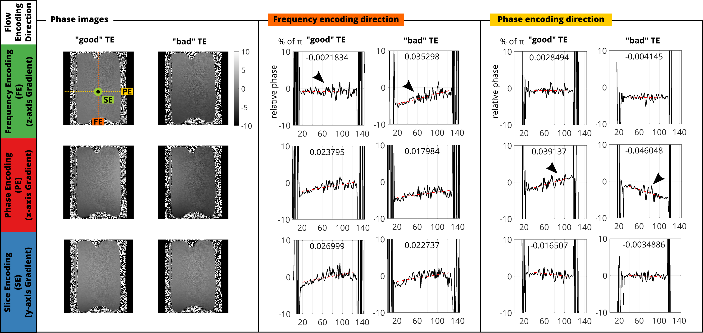
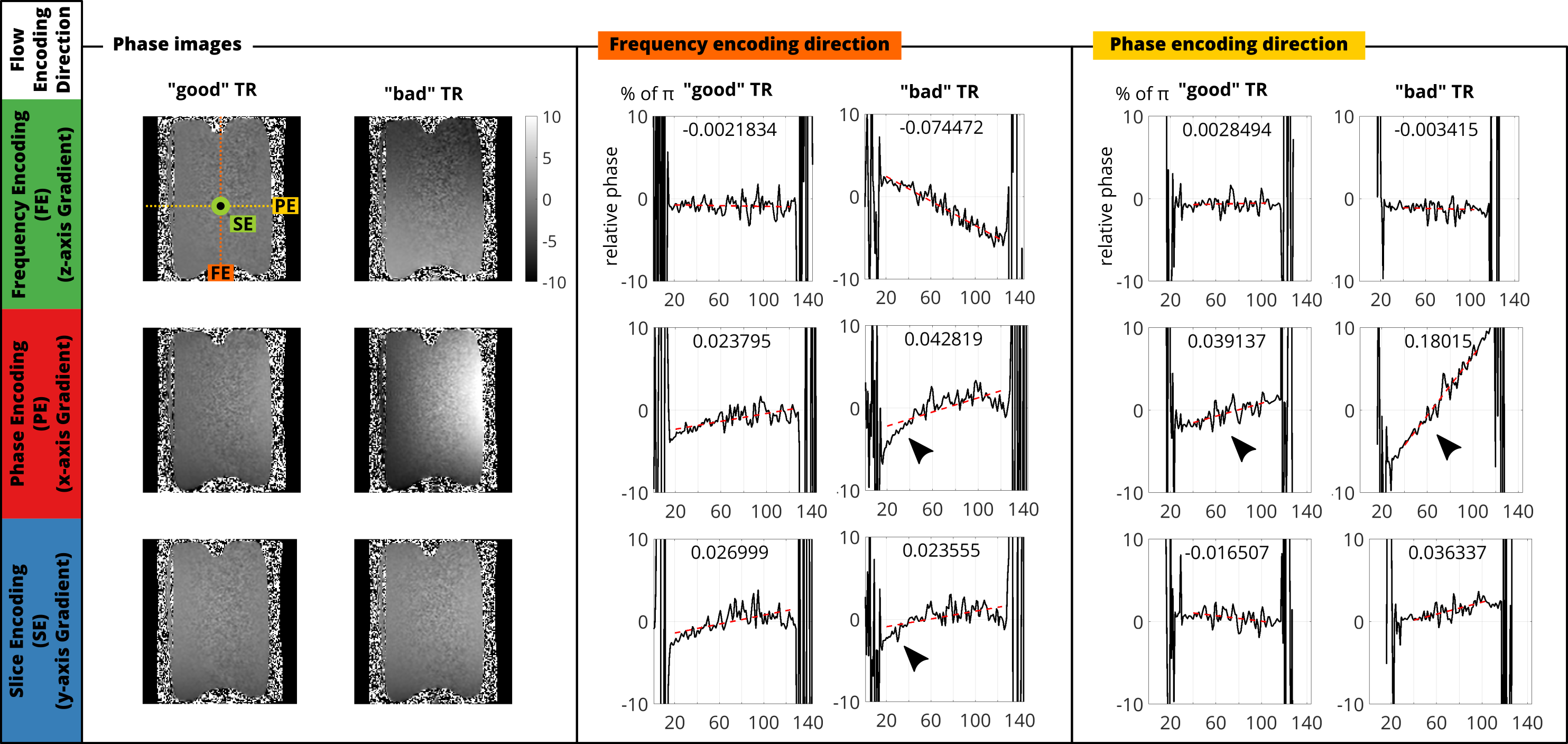
In order to quantify the image phase, a polynomial of first order was fitted to 1D centered profiles along frequency and phase encoding direction and resulted in a slope (Figure3,4; red broken lines, value given in the plots) for each$$$\;\mathrm{TE},\mathrm{TR}$$$.
Results & Discussion
Figure3 presents the spatial phase evolution for fixed$$$\;\mathrm{TR}=5\mathrm{ms}\;$$$($$$\;f_{res}=1065\mathrm{Hz}\;$$$not on frequency comb, Figure 1C) and compares$$$\;\mathrm{TE}=2.35\mathrm{ms}\;$$$(good) vs.$$$\;\mathrm{TE}=2.97\mathrm{ms}\;$$$(bad). Depending on the flow encoding direction, increased slopes of the first order fit result are noted in the corresponding profile direction. Orthogonal profiles do not differ between TEs.Figure4 presents the spatial phase evolution for fixed$$$\;\mathrm{TE}=2.35\mathrm{ms}\;$$$and compares$$$\;\mathrm{TR}=5\mathrm{ms}\;$$$(good) vs.$$$\;\mathrm{TR}=4.69\mathrm{ms}\;$$$(bad). The slope is increased in phase encoding direction between good and bad$$$\;\mathrm{TR}\;$$$(x3.6). Flow encoding in phase and slice encoding direction results in quadratic background phase in frequency encoding direction.
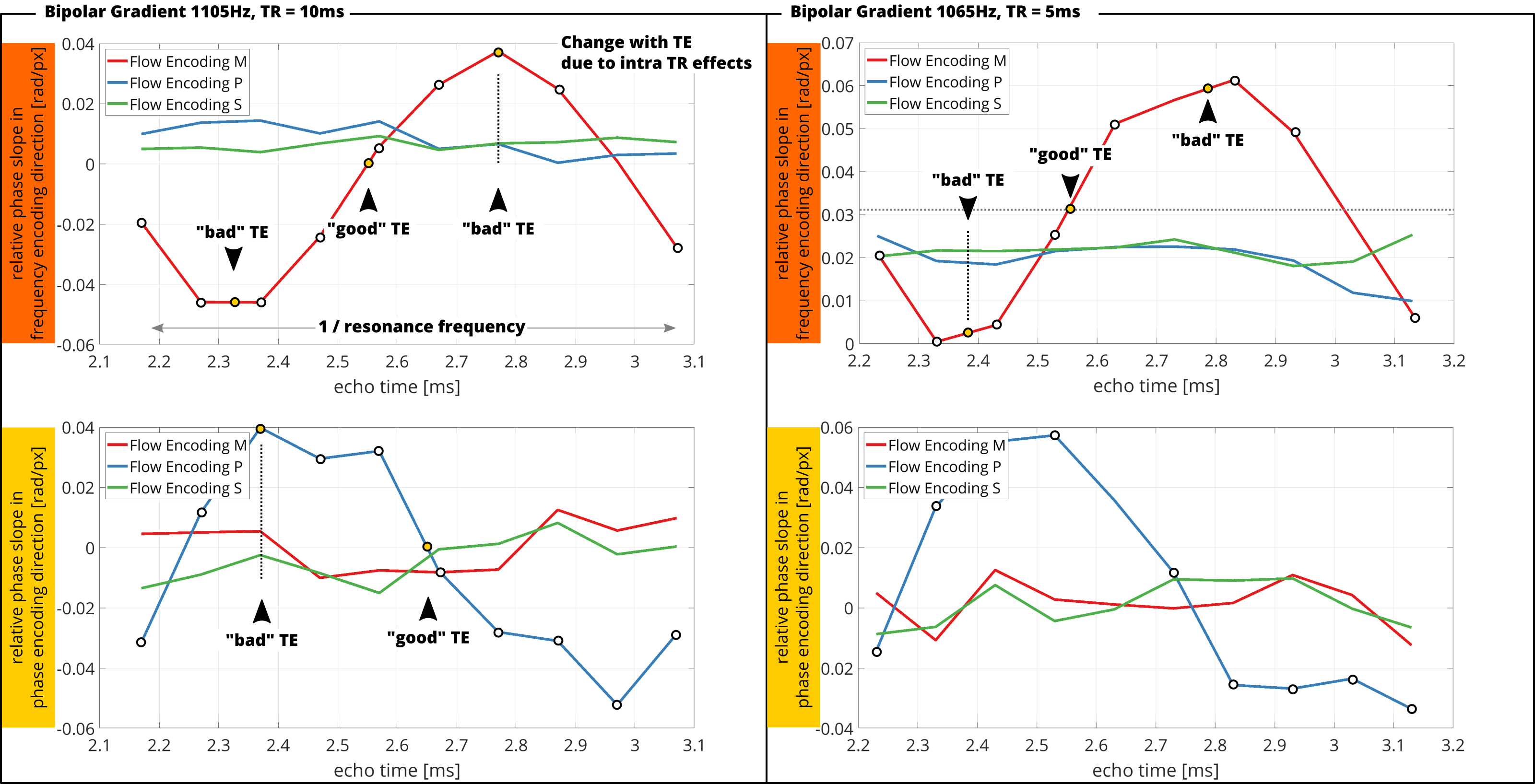
In Figure5, the slope of the fit is presented for varying TEs and two MEG frequencies 1105Hz and 1065Hz with$$$\;\mathrm{TR}=10\mathrm{ms}\;$$$and$$$\;\mathrm{TR}=5\mathrm{ms}\;$$$, respectively. Only the phase profile in flow-encode direction changes its slope. The period of the change is given by$$$\;1/f_{res}\;$$$and complies to Figure1A. We find increased slopes of up to 15-fold when comparing “good” to “bad” TE.
Conclusion
In this work, we identified mechanical resonances as a source of erroneous background phases when using PC-MRI. By mapping mechanical resonances using simple audio recordings before imaging, we were able to identify beneficial combinations of TR and TE for which the background phase error was kept minimal. For suboptimal choices of TR, the spatial background phase resulted in quadratic dependencies. By shifting$$$\;\mathrm{TE}\;$$$by$$$\;0.6\mathrm{ms}\;$$$ or$$$\;\mathrm{TR}\;$$$by$$$\;0.31\mathrm{ms}\;$$$, we were able to achieve a minimal background phase. For future MRI systems, audio recordings could be used to track mechanical resonance frequencies during short preparation phases to fine-tune sequence parameters.Acknowledgements
The authors acknowledge funding of the Platform for Advanced Scientific Computing of the Council of Federal Institutes of Technology (ETH Board), Switzerland.References
1. Gatehouse P, Rolf M, Graves M, et al. Flow measurement by cardiovascular magnetic resonance: A multi-centre multi-vendor study of background phase offset errors that can compromise the accuracy of derived regurgitant or shunt flow measurements. J. Cardiovasc. Magn. Reson. 2010;12:1–8 doi: 10.1186/1532-429X-12-5.
2. Giese D, Haeberlin M, Barmet C, Pruessmann KP, Schaeffter T, Kozerke S. Analysis and correction of background velocity offsets in phase-contrast flow measurements using magnetic field monitoring. Magn. Reson. Med. 2012;67:1294–1302 doi: 10.1002/mrm.23111.
3. Rolf MP, Hofman MBM, Gatehouse PD, et al. Sequence optimization to reduce velocity offsets in cardiovascular magnetic resonance volume flow quantification - A multi-vendor study. J. Cardiovasc. Magn. Reson. 2011;13:1–10 doi: 10.1186/1532-429X-13-18.
4. Busch J, Giese D, Kozerke S. Image-based background phase error correction in 4D flow MRI revisited. J. Magn. Reson. Imaging 2017;46:1516–1525 doi: 10.1002/jmri.25668.
5. Guenthner C, Sethi S, Troelstra M, Dokumaci AS, Sinkus R, Kozerke S. Ristretto MRE: A generalized multi-shot GRE-MRE sequence. NMR Biomed. 2019;32:1–13 doi: 10.1002/nbm.4049.
Figures