0275
XPDNet for MRI Reconstruction: an application to the 2020 fastMRI challenge1Neurospin, Gif-Sur-Yvette, France, 2Cosmostat team, CEA, Gif-Sur-Yvette, France, 3Parietal team, Inria Saclay, Gif-Sur-Yvette, France
Synopsis
We present a new neural network, the XPDNet, for MRI reconstruction from periodically under-sampled multi-coil data. We inform the design of this network by taking best practices from MRI reconstruction and computer vision. We show that this network can achieve state-of-the-art reconstruction results, as shown by its ranking of second in the fastMRI 2020 challenge.
Introduction
The acceleration of the scan time of Magnetic Resonance Imaging (MRI) can be done using Compressed Sensing (CS)1 and Parallel Imaging (PI)2,3. To have access to the underlying anatomical object $$$x\in\mathbb{C}^{n \times n}$$$, one must solve the following idealized inverse problem for all coils:$$M_{\Omega} F S_\ell x = y_\ell, \quad \forall \ell=1,\ldots, L$$
where $$$M_{\Omega}\in\{0,1\}^{n\times n}$$$ is a mask indicating which points in the Fourier space (also called k-space) are sampled, $$$S_\ell\in\mathbb{C}^{n\times n}$$$ is a sensitivity map for coil $$$\ell$$$, $$$F$$$ is the 2D Fourier transform, and $$$y_\ell\in\mathbb{C}^{n \times n}$$$ is the k-space measurement for coil $$$\ell$$$. This is typically solved with optimization algorithms that introduce a regularisation term to cope with indeterminacy.
$$argmin \sum_{\ell=1}^L \frac{1}{2} \|y_\ell-M_{\Omega} F S_\ell x \|_{2}^{2}+R(x)$$
The places where learning could improve the quality and the speed of the reconstruction are:
- the optimization algorithm hyper-parameters like step sizes and momentum;
- the sensitivity maps $$$(S_{\ell})_\ell$$$, usually estimated using ESPIRiT4;
- the regularizer $$$R(x)$$$, usually $$$\lambda \|\psi x\|_1$$$ where $$$\psi$$$ is the decomposition over some wavelet basis;
- the data consistency term $$$\sum_{\ell=1}^L \frac{1}{2}\left\|y_{\ell}-M_{\Omega} F S_{\ell} x\right\|_{2}^{2}$$$, usually derived from an additive white Gaussian noise model.
Methods
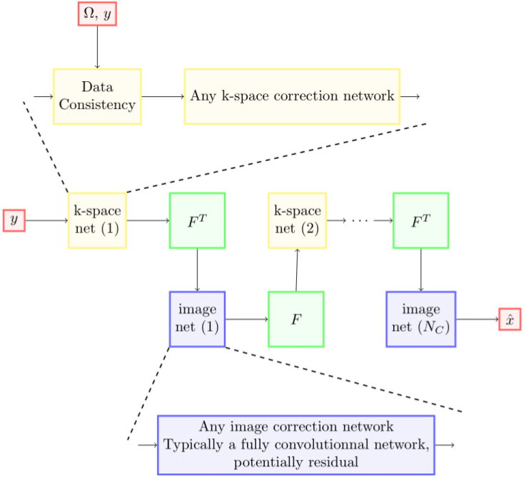
Cross-domain networks. The general intuition behind cross-domain networks is that we are going to alternate the correction between the image space and the measurements space. The key tool for that is the unrolling of optimisation algorithms5. An illustration of what cross-domain networks generally look like is provided in Fig. 1.Unrolling the PDHG. The XPDNet is a particular instance of cross-domain networks. It is inspired by the PDNet6 which unrolls the Primal Dual Hybrid Gradient (PDHG) algorithm7. In particular, a main feature of the PDNet is its ability to learn the optimisation parameters using a buffer of iterates, here of size 5.
Image correction network. The plain Convolutional Neural Network (CNN) of the original PDNet is replaced by a Multi-scale Wavelet CNN (MWCNN)8, but the code allows for it to be any denoiser, hence the presence of X in its name. We chose to use a smaller image correction network than that presented in the original paper8, in order to afford more unrolled iterations in memory9.
k-space. In this challenge, since the data is multi-coil, we did not use any k-space correction network which would be very demanding in terms of memory footprint. However, we introduced a refinement network10 for $$$S$$$, initially estimated from the lower frequencies of the retrospectively under-sampled coil measurements. This sensitivity maps refiner10 is chosen to be a simple U-net11.
We therefore have 25 unrolled iterations, an MWCNN that has twice as less filters in each scale, a small sensitivity maps refiner and no k-space correction network.
Training details. The loss used for the network training was a compound loss12, consisting of a weighted sum of an $$$L1$$$ loss and the multi-scale SSIM (MSSIM)13. The optimizer was the Rectified ADAM (RAdam)14 with default TensorFlow parameters. The training was carried for 100 epochs (batch size of 1) and separately for acceleration factors 4 and 8. The networks were then fine-tuned for each contrast for 10 epochs. On a single V100 GPU, the training lasted 1 week for each acceleration.
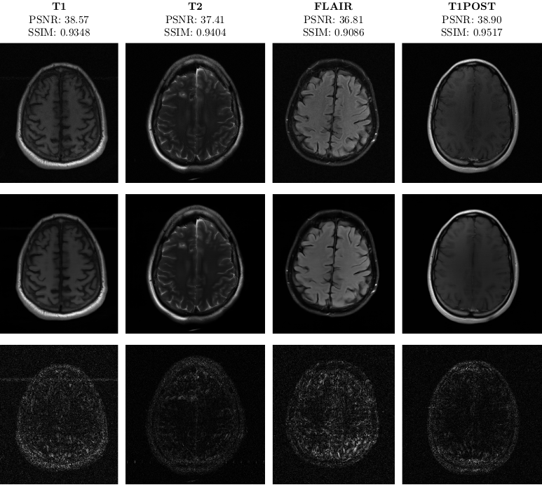
Data. The network was trained on the brain part of the fastMRI dataset15. The training set consists of 4,469 volumes from 4 different contrasts: T1, T2,FLAIR and T1 with admissions of contrast agent (labelled T1POST). The validation was carried over 30 contrast-specific volumes from the validation set.
Results
Quantitative. We used the PSNR and SSIM metrics to quantitatively compare the reconstructed magnitude image and the ground truth. They are given for each contrast and for the 2 acceleration factors in the Figs. 2- 3. Similar results are available on the public fastMRI leaderboard, although generally slightly better. It is a bit difficult to consider these results when compared to only the zero-filled metrics, but these quantitative metrics do not accurately capture the performance of the GRAPPA algorithm2. However, at the time of submission, this approach ranks second in the fastMRI leaderboards for the PSNR metric, and finished second in the 4× and 8× tracks of the fastMRI 2020 brain reconstruction challenge16.Qualitative.The visual inspection of the images reconstructed (available in Fig. 2) at acceleration factor 4 shows little to no visible difference with the ground truth original image. However, when increasing the acceleration factor to 8, we can see that smoothing starts to appear which leads to a loss of structure as can be seen in Fig. 3.
Conclusion and Discussion
We managed to gather insights from many different works on computer vision and MRI reconstruction to build a modular approach. Currently our solution XPDNet is among the best in PSNR and NMSE for both the multi-coil knee and brain tracks at the acceleration factors 4 and 8. Furthermore, the modularity of the current architecture allows to use the newest denoising architectures when they become available. However, the fact that this approach fails to outperform the others on the SSIM metric is to be investigated in further work.Acknowledgements
We acknowledge the financial support of the Cross-Disciplinary Program on Numerical Simulation of CEA, the French Alternative Energies and Atomic Energy Commission for the project entitled SILICOSMIC.
We also acknowledge the French Institute of development and ressources in scientific computing (IDRIS) for their AI program allowing us to use the Jean Zay supercomputers’ GPU partitions.
References
1. Michael Lustig, David Donoho, and John M. Pauly. “Sparse MRI: The Application of Compressed Sensing for Rapid MR Imaging Michael”. In:Magnetic Resonance in Medicine (2007).issn: 10014861.doi:10.1002/mrm.21391.
2. Mark A Griswold et al. “Generalized Autocalibrating Partially Parallel Acquisitions (GRAPPA)”. In:Magnetic Resonance in Medicine 47 (2002),pp. 1202–1210.doi:10.1002/mrm.10171.url:www.interscience.wiley.com.
3. Klaas P. Pruessmann et al. “SENSE: Sensitivity encoding for fast MRI”. In:Magnetic Resonance in Medicine 42.5 (1999), pp. 952–962.issn: 07403194.doi:10.1002/(SICI)1522-2594(199911)42:5<952::AID-MRM16>3.0.CO;2-S.
4. Martin Uecker et al. “ESPIRiT-An Eigenvalue Approach to AutocalibratingParallel MRI: Where SENSE meets GRAPPA HHS Public Access”. In:Magn Reson Med 71.3 (2014), pp. 990–1001.doi:10.1002/mrm.24751.
5. Karol Gregor and Yann Lecun. “Learning Fast Approximations of SparseCoding”. In:Proceedings of the 27th International Conference on Machine Learning. 2010.
6. Jonas Adler and Ozan Öktem. “Learned Primal-Dual Reconstruction”. In:IEEE Transactions on Medical Imaging 37.6 (2018), pp. 1322–1332.issn:1558254X.doi:10.1109/TMI.2018.2799231.
7. Antonin Chambolle and Thomas Pock. “A First-Order Primal-Dual Al-gorithm for Convex Problems with Applications to Imaging”. In: (2011),pp. 120–145.doi:10.1007/s10851-010-0251-1.
8. Pengju Liu et al.Multi-level Wavelet-CNN for Image Restoration. Tech. rep.2018.url:https://arxiv.org/pdf/1805.07071.pdf.
9. Zaccharie Ramzi, Philippe Ciuciu, and Jean Luc Starck. “Benchmarking MRI reconstruction neural networks on large public datasets”. In:Applied Sciences (Switzerland)10.5 (2020).issn: 20763417.doi:10.3390/app10051816.
10. Anuroop Sriram et al.End-to-End Variational Networks for Accelerated MRI Reconstruction. Tech. rep. 2020.
11. Olaf Ronneberger, Philipp Fischer, and Thomas Brox. “U-Net: Convolutional Networks for Biomedical Image Segmentation”. In:International Conference on Medical image computing and computer-assisted intervention.2015, pp. 234–241.url:http://lmb.informatik.uni-freiburg.de/.
12. Nicola Pezzotti et al.An Adaptive Intelligence Algorithm for Undersampled Knee MRI Reconstruction: Application to the 2019 fastMRI Challenge.Tech. rep. 2020.
13. Zhou Wang et al. “Image Quality Assessment: From Error Visibility to Structural Similarity”. In:IEEE TRANSACTIONS ON IMAGE PRO-CESSING13.4 (2004).doi:10.1109/TIP.2003.819861.url:http://www.cns.nyu.edu/~lcv/ssim/..
14. Liyuan Liu et al. “On the Variance of the Adaptive Learning Rate and Beyond”. In:Proceedings of International Conference for Learning Representations(2020), pp. 1–3.
15. Jure Zbontar et al.fastMRI: An Open Dataset and Benchmarks for Accelerated MRI. Tech. rep. 2018.url:https://arxiv.org/pdf/1811.08839.pdf.5
16. Matthew J. Muckley et al.State-of-the-art Machine Learning MRI Re-construction in 2020: Results of the Second fastMRI Challenge. Tech. rep.2020, pp. 1–16. url:http://arxiv.org/abs/2012.06318.6
Figures