0274
Compressed Sensing MRI Revisited: Optimizing $$$\ell_{1}$$$-Wavelet Reconstruction with Modern Data Science Tools1Electrical Engineering, University of Minnesota, Minneapolis, MN, United States, 2Center for magnetic resonance research, Minneapolis, MN, United States, 3University of Minnesota, Minneapolis, MN, United States
Synopsis
Deep learning (DL) has shown great promise in improving the reconstruction quality of accelerated MRI. These methods are shown to outperform conventional methods, such as parallel imaging and compressed sensing (CS). However, in most comparisons, CS is implemented with ~2-3 empirically-tuned hyperparameters. On the other hand, DL methods enjoy a plethora of advanced data science tools. In this work, we revisit l1 -regularized CS using these modern tools. Using an unrolled ADMM approach, we show that classical l1-wavelet CS can achieve comparable quality to DL reconstructions, with only 116 parameters compared to hundreds of thousands for the DL approaches.
INTRODUCTION
Recently, many deep learning (DL) methods have been developed for accelerated MRI1-6 showing improved performance over conventional methods, such as parallel imaging and compressed sensing (CS). Among these, physics-guided DL (PG-DL), which unrolls conventional optimization algorithms that incorporate the encoding operator have received interest. Unlike CS, which uses a linear representation of images as part of regularization, PG-DL utilizes a non-linear representation that is implicitly learned through a convolutional neural network (CNN) for regularization. DL methods are trained over large databases, include a large number of parameters, often more than hundreds of thousands2,7,8, use sophisticated optimization algorithms9, and advanced loss functions10. On the other hand, when CS reconstruction methods are implemented for comparison, they typically use two-to-three parameters, which are hand-tuned empirically. While there are some automatic tuning efforts11,12, these have not leveraged the modern data science tools that have become available in the DL era. In this work, we revisit $$$\ell_{1}$$$-wavelet CS for accelerated MRI using these data science tools. We use an unrolled ADMM algorithm, with only 4 orthogonal wavelets, and train it end-to-end similar to PG-DL methods. Results on knee MRI show the optimized CS method performs closely with advanced PG-DL methods, while only having 116 tunable parameters and using a linear representation for interpretable and convex sparse image processing.METHODS
Inverse Problem for Accelerated MRI: Following objective function is solved in accelerated MRI$$\arg \min _{\mathbf{x}} \frac{1}{2}\left\|\mathbf{y}_{\Omega}-\mathbf{E}_{\Omega} \mathbf{x}\right\|_{2}^{2}+\mathcal{R}(\boldsymbol{x}).(1)$$where $$$\mathbf{y}_{\Omega}$$$ is multi-coil k-space with undersampling pattern Ω, $$$\mathbf{E}_{\boldsymbol{\Omega}}$$$ is forward multi-coil encoding operator,$$$\left\|\mathbf{y}_{\Omega}-\mathbf{E}_{\Omega} \mathbf{x}\right\|_{2}^{2}$$$ enforces data consistency (DC) and $$$\mathcal{R}(.)$$$ is a regularizer. In conventional CS, $$$\mathcal{R}(x)$$$ is chosen as weighted $$$\ell_{1}$$$-norm of transform coefficients in a pre-specified domain14,15,16 This objective function is solved via an iterative optimization algorithm17.These algorithms are typically run until a convergence criterion is met, making hyperparameter tuning difficult.On the other hand,in PG-DL reconstruction,the iterative optimization algorithm is unrolled for a fixed number of iterations18,19. These typically decouple the solution to a series of regularizer and DC units. In PG-DL, the regularizer is implemented implicitly via CNNs, while the DC unit uses linear methods like conjugate-gradient (CG)3. The network is trained end-to-end$$\min _{\boldsymbol{\theta}} \frac{1}{N} \sum_{i=1}^{N} \mathcal{L}\left(\mathbf{y}_{r e f}^{i}, \mathbf{E}_{f u l l}^{i}\left(f\left(\mathbf{y}_{\Omega}^{i}, \mathbf{E}_{\Omega}^{i} ; \boldsymbol{\theta}\right)\right)\right).(2)$$where $$$\mathbf{y}_{r e f}^{i}$$$ is fully-sampled reference k-space of $$$i^{\text {th }}$$$ subject, $$$f\left(\mathrm{y}_{\Omega}^{i}, \mathbf{E}_{\Omega}^{i} ; \boldsymbol{\theta}\right)$$$ denotes network output with parameters $$$\theta$$$ for $$$i^{\mathrm{th}}$$$ subject, $$$\mathbf{E}_{f u l l}^{i}$$$ is fully-sampled multi-coil encoding operator, N is number of datasets, and $$$\mathcal{L}(\ldots)$$$ is training loss.Proposed Optimized -Wavelet CS Reconstruction: To optimize conventional CS reconstruction, we utilize the data science tools employed by PG-DL methods. We set $$$\mathcal{R}(\boldsymbol{x})=\sum_{\mathbf{n}=1}^{\mathbf{N}} \mathbf{\mu}_{\mathbf{n}}\left\|\mathbf{W}_{\mathbf{n}} \mathbf{x}\right\|_{1}$$$, where $$$\mathbf{W}_{\mathbf{n}}$$$ are orthogonal discrete wavelet transforms. This objective function is solved via ADMM, which is unrolled for T iterations (Fig. 1). For ADMM, unrolling leads to three tunable parameters for $$$\ell_{1}$$$ soft-thresholding, augmented Lagrangian relaxation and dual update, per unrolled iteration and wavelet. These parameters are trained end-to-end using the objective function in Eq. (2).The proposed approach was implemented with N=4 wavelets, corresponding to Daubechies1-4 orthonormal wavelets. T=10 unrolls were used. Adam optimizer with learning rate 5×10⁻³ was used for training over 100 epochs, with a mixed normalized $$$ \ell_{1}-\ell_{2}$$$ loss6. DC sub-problem for ADMM was solved using CG3 with 5 iterations and warm-start.Imaging Datasets: Fully-sampled coronal proton density (PD) with and without fat-suppression (PD-FS) knee data were obtained from the NYU-fastMRI database13. The datasets were retrospectively under-sampled with a random mask (R=4, 24 ACS lines). Training was performed on 300 slices from 10 subjects. Testing was performed on 10 different subjects. The proposed approach was compared with PG-DL based on ADMM unrolling4 that utilized a ResNet-based regularizer unit, which has been used in recent studies7,20. Note this constitutes a head-to-head comparison, with the only difference in the $$$\mathcal{R}(\cdot)$$$ term, where our approach uses $$$\ell_{1}$$$-norm of wavelets for solving a convex problem, while the other uses a CNN for implicit regularization. Further comparisons were also made with CG-SENSE20. Results were quantitatively evaluated using SSIM and NMSE.RESULTS
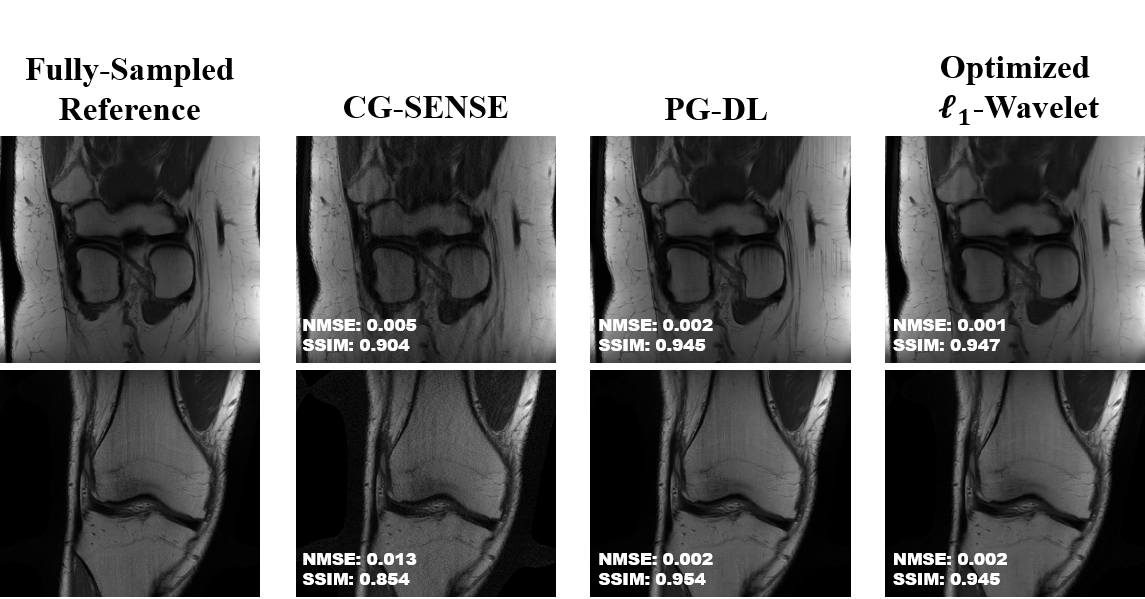
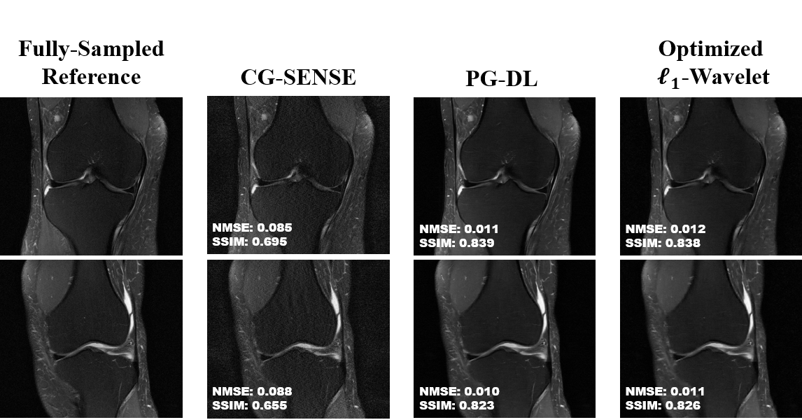
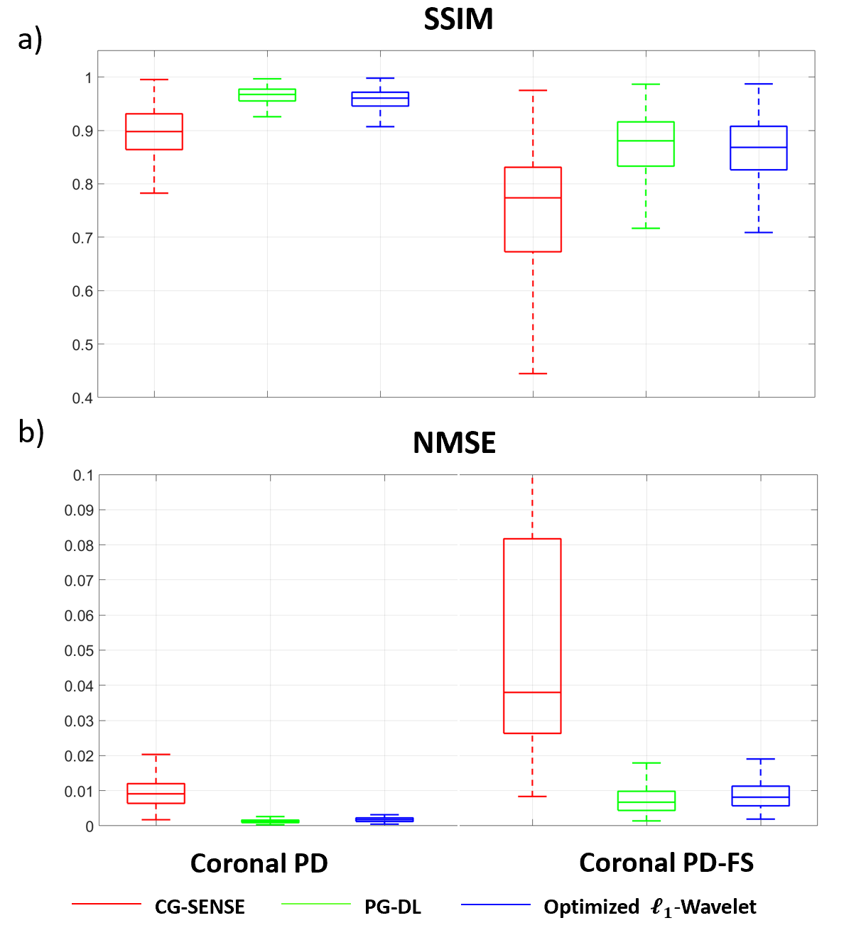
Fig. 2 shows results for representative coronal PD slices. Both PG-DL and the optimized $$$\ell_{1}$$$ -wavelet CS remove aliasing artifacts visible in CG-SENSE, with similar quantitative metrics. Fig. 3 displays results for coronal PD-FS knee data. The optimized $$$\ell_{1}$$$ -wavelet CS again has similar quality to PG-DL both visibly and quantitatively. Fig. 4 summarizes quantitative results from knee MRI, where the proposed CS approach performs closely with PG-DL.DISCUSSION AND CONCLUSIONS
In this study, we revisited $$$\ell_{1}$$$-wavelet CS for accelerated MRI using modern data science tools for fine-tuning. As expected, PG-DL outperformed our method, but the performance gap was much smaller than previously published literature. This is interesting for a number of reasons: 1)PG-DL uses complicated non-linear representations with huge number of parameters. Our wavelet-based representation is linear, interpretable, involves few parameters and allows convex optimization. There is <0.01 difference in SSIM between a 116-parameters wavelet and a >500,000-parameters PG-DL approach. 2)While PG-DL can be further improved with more advanced neural networks and training strategies21, our CS approach used one of the simplest linear models described by fixed orthogonal wavelets, and involved no learning of the representation.Further gains for CS may be possible via learning linear representations/frames22,23, which warrants investigation.Acknowledgements
Grant support: NIH R01HL153146, NIH P41EB027061, NIH U01EB025144; NSF CAREER CCF-1651825References
1.Wang S, Su Z, Ying L, Peng X, Zhu S, Liang F, Feng D, Liang D. Accelerating magnetic resonance imaging via deep learning. IEEE 13th International Symposium on Biomedical Imaging (ISBI); 2016. p 514-517.
2.Hammernik K, Klatzer T, Kobler E, Recht MP, Sodickson DK, Pock T, Knoll F. Learning a variational network for reconstruction of accelerated MRI data. Magnetic Resonance in Medicine 2018;79(6):3055-3071.
3.Aggarwal HK, Mani MP, Jacob M. MoDL: Model-Based Deep Learning Architecture for Inverse Problems. IEEE Trans Med Imaging 2019;38(2):394-405.
4.Yang Y, Sun J, Li H, Xu Z. Deep ADMM‐Net for compressive sensing MRI. Advances in neural information processing systems (NIPS);2016:10–18.
5.Schlemper J, Caballero J, Hajnal JV, Price AN, Rueckert D. A Deep Cascade of Convolutional Neural Networks for Dynamic MR Image Reconstruction. IEEE Transactions on Medical Imaging 2018;37(2): 491-503.
6.Knoll F, Hammernik K, Zhang C, Moeller S, Pock T, Sodickson DK, Akcakaya M. Deep Learning Methods for Parallel Magnetic Resonance Image Reconstruction. arXiv preprint arXiv:1904.01112; 2019.
7.Yaman B, Hosseini SA, Moeller S, Ellermann J, Uğurbil K, Akçakaya M. Self‐supervised learning of physics‐guided reconstruction neural networks without fully sampled reference data. Magnetic Resonance in Medicine 2020;84(6):3172-3191.
8.Sriram A, Zbontar J, Murrell T, Defazio A, Zitnick C L, Yakubova N, Knoll F, Johnson P. End-to-End Variational Networks for Accelerated MRI Reconstruction. Medical Image Computing and Computer Assisted Intervention – MICCAI 2020 Lecture Notes in Computer Science;2020: 64-73.
9.Zou F, Shen L, Jie Z, Zhang W, Liu W. A Sufficient Condition for Convergences of Adam and RMSProp. Proceedings of the IEEE/CVF Conference on Computer Vision and Pattern Recognition (CVPR);2019: 11127-11135
10.Mardani M, Gong E, Cheng J Y, Vasanawala S S, Zaharchuk G, Xing L, Pauly J M. Deep Generative Adversarial Neural Networks for Compressive Sensing MRI. IEEE Transactions on Medical Imaging 2019;38(1):167-179.
11.Shahdloo M, Ilicak E, Tofighi M, Saritas EU, Cetin AE, Cukur T. Projection onto Epigraph Sets for Rapid Self-Tuning Compressed Sensing MRI. IEEE Transactions on Medical Imaging 2019;38(7):1677-1689.
12.Ramani S, Liu Z, Rosen J, Nielsen JF, Fessler JA. Regularization parameter selection for nonlinear iterative image restoration and MRI reconstruction using GCV and SUREbased methods. IEEE Trans actions on Image Processing 2012;21(8):3659-3672.
13.Knoll F, Zbontar J, Sriram A, et al. fastMRI: A publicly available raw k‐space and DICOM dataset of knee images for accelerated MR Image reconstruction using machine learning. Radiology Artificial Intelligence 2020;2:e190007.
14.Donoho DL, Compressed sensing. IEEE Transactions on Information Theory 2006.;52(4):1289-1306.
15.Candes EJ, Romberg J, Tao T. Robust uncertainty principles: exact signal reconstruction from highly incomplete frequency information, IEEE Transactions on Information Theory 2006;52(2):489-509.
16.Lustig M, Donoho D, Pauly JM. Sparse MRI: The application of compressed sensing for rapid MR imaging. Magnetic Resonance in Medicine 2007;58(6):1182-1195.
17.Fessler JA. Optimization Methods for Magnetic Resonance Image Reconstruction: Key Models and Optimization Algorithms. IEEE Signal Processing Magazine 2020;37(1):33-40.
18.Gregor K, LeCunY. Learning fast approximations of sparse coding. ICML 2010 - Proceedings, 27th International Conference on Machine Learning;2010:399-406.
19.Monga V, Li Y, Eldar YC. Algorithm unrolling: Interpretable efficient deep learning for signal and image processing. arXiv preprint arXiv:1912.10557; 2019.
20.Hosseini SA, Yaman B, Moeller S, Hong M, Akcakaya M. Dense Recurrent Neural Networks for Accelerated MRI: History-Cognizant Unrolling of Optimization Algorithms. IEEE Journal of Selected Topics in Signal Processing 2020;14(6):1280-1291.
21.Muckley MJ et al. State-of-the-art Machine Learning MRI Reconstruction in 2020: Results of the Second fastMRI Challenge. arXiv preprint arXiv:2012.06318; 2020.
22.Wen B, Ravishankar S, Pfister L, Bresler Y. Transform Learning for Magnetic Resonance Image Reconstruction: From Model-Based Learning to Building Neural Networks. IEEE Signal Processing Magazine 2020;37(1):41-53.
23.Akcakaya M, Tarokh V. A Frame Construction and a Universal Distortion Bound for Sparse Representations. IEEE Transactions on Signal Processing 2008;56(6):2443-2450.
Figures