Introduction

Recently, deep learning (DL)-based methods have become popular in image reconstruction and shown great potential in significantly speeding up MR imaging^1,2. However, existing DL-based works for MR reconstruction mainly have explicit data consistency under the assumption that the noise distribution follows the zero mean normal distribution. In practice, the distribution of the noise is more complicated than the zero mean normal distribution. In this work, we propose a novel reconstruction approach that uses a data likelihood model learned by deep networks, which we term as Learned DC reconstruction. Compared to other DL-based methods, the main difference of Learned DC is the powerful data likelihood that can capture the distribution of imaging noise.

Theory

The forward imaging model of MRI can be formulated as $$ f=Ax+\delta (1) $$ where $$$m\in C^N$$$ is the vector of pixels we wish to reconstruct from the k-space data $$$f\in C^M$$$, $$$\delta$$$ denotes the measurement error, which can be well modeled as noise, $$$A:C^N\mapsto C^M$$$ is the encoding matrix, with $$$N\geq M$$$.
The problem of reconstruction is often formulated as a MAP estimation, where the goal is to maximize the posterior probability. Assuming the measurement error $$$\delta$$$ is zero mean, normal distributed and uncorrelated additive, the reconstruction problem can be written as $$arg\min_{m}||Am-f||_2^2+\lambda R(m) (2) $$ The regularization term $$$R(m)$$$ is corresponding to the prior information of the image which is learned by deep networks.
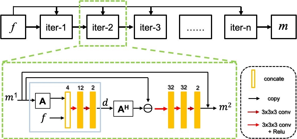
While in reality, the zero mean uncorrelated additive normal distribution is not suitable for modeling the noise distribution because of the accumulation of noise from coils and bodies and the electronic noise. Hence, we assume that the measured noise satisfies the exponential distribution after a nonlinear transform. Therefore, the data likelihood follows $$p(f|m)\sim e^{-F(Am,f)} (3)$$ where $$$F(Am,f) $$$is the nonlinear mapping that transfers the measurement error distribution to the exponential distribution. Then the reconstruction problem can be written as $$\widetilde{m}=arg\min_m[F(Am,f)+R(m)] (4)$$ The minimization problem of (4) can be solved via the proximal gradient descent algorithm as follows $$ \begin{cases}z=m^{n-1}-\tau \triangledown F(Am^{n-1},f)\\m^n=prox_{R,\tau}(z)\end{cases} (5)$$ where $$$\triangledown$$$ denotes the gradient (or sub-gradient) of $$$F(Am,f)$$$. We replace the proximal operator with the learned operator $$$\Lambda$$$ and a parameterized operator $$$g$$$ is referred to $$$\triangledown F(Am,f)$$$, the whole iteration can be rewritten as $$ \begin{cases}d=g(Am^{n-1},f)\\m^n=\Lambda(m^{n-1}-A^Hd)\end{cases} (6)$$ The illustrative diagram of the proposed Learned DC for dynamic imaging is shown in Figure 1. Each iteration of reconstruction accepts the multi-coil undersampled k-space data $$$f$$$ and coil-combined image $$$m$$$ as input.

Method

Dynamic cardiac cine data was used to evaluate the feasibility of the proposed Learned DC. The fully sampled cardiac cine data were collected from 29 healthy volunteers on a 3T scanner (MAGNETOM Trio, Siemens Healthcare, Erlangen, Germany) with 20-channel receiver coil arrays. Informed consent was obtained from the imaging subjects in compliance with the Institutional Review Board (IRB) policy. For each subject, 10 to 13 short-axis slices were imaged with the retrospective electrocardiogram (ECG)-gated segmented bSSFP sequence during breath-hold. With data augmentation and shear, we obtained 800 2D-t multi-coil cardiac MR data of size 192×192×18 (x×y×t) for training and 118 for testing. The variable density incoherent spatiotemporal acquisition (VISTA) sampling mask³ was used to demonstrate the performance of reconstruction methods. The coil sensitivity maps were calculated from the fully-filled, time-averaged k-space center using ESPIRiT⁴.

Results

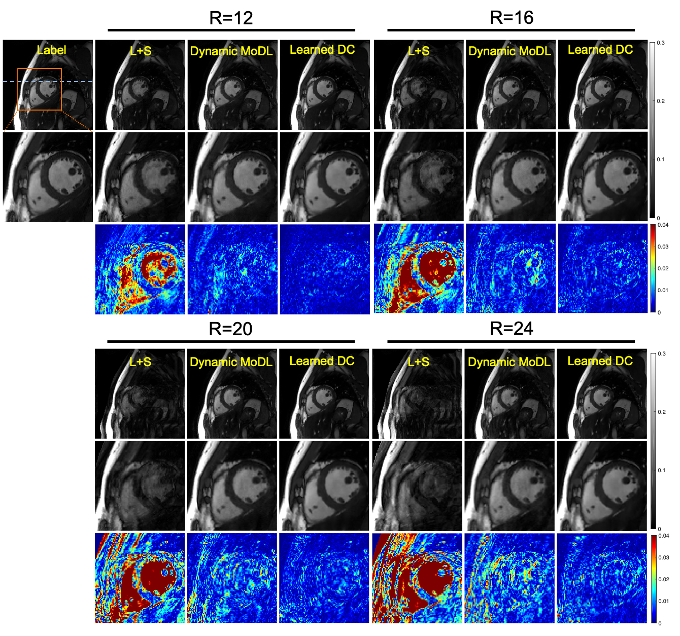
We compared our proposed approach with different dynamic MR reconstruction methods, including state-of-the-art compressed sensing method L+S⁵, and DL-based method dynamic MoDL⁶.
The qualitative comparisons with high acceleration factors are shown in Figure 2. The reconstructed images in the spatial domain, as well as the corresponding error maps were provided. The DL methods (dynamic MoDL and Learned DC) achieve better performance than the conventional CS method L+S due to the learned image prior. The proposed Learned DC can faithfully reconstruct the images with smaller errors and clearer anatomical details indicated by the error maps and the zoom-in images. Even for the extremely high acceleration factor of 24, the proposed Learned DC can provide excellent reconstruction with aliasing artifacts removing and detail preserving.
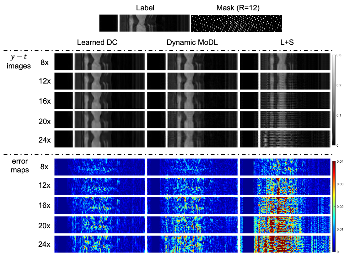
Figure 3 shows the reconstructions of different methods along the temporal dimension with different acceleration factors. It can be observed that our proposed approach can still recover the dynamic information very well on extremely high undersampled data (R=24), where the conventional CS approach fails and the competing deep learning approach does not well in artifact removing.

Conclusion

In this work, we have proposed a novel DL-based approach to approximate the data likelihood and learn the image prior. Experimental results on dynamic imaging show the superior performance of the proposed approach.

Acknowledgements

This work was supported in part by the National Key R&D Program of China (2017YFC0108802 and 2017YFC0112903); National Natural Science Foundation of China (61771463, 81830056, U1805261, 81971611, 61871373, 81729003, 81901736); Natural Science Foundation of Guangdong Province (2018A0303130132); Key Laboratory for Magnetic Resonance and Multimodality Imaging of Guangdong Province; Shenzhen Peacock Plan Team Program (KQTD20180413181834876); Innovation and Technology Commission of the government of Hong Kong SAR (MRP/001/18X); Strategic Priority Research Program of Chinese Academy of Sciences (XDB25000000)