0230

Design of slice-selective RF pulses using deep learning

Felix Krüger¹, Max Lutz¹, Christoph Stefan Aigner¹, and Sebastian Schmitter¹
¹Physikalisch-Technische Bundesanstalt, Braunschweig and Berlin, Germany

Synopsis

We utilize a residual neural network for the design of slice-selective RF and gradient trajectories. The network was trained with 300k SLR RF pulses. The network predicts the RF pulse and the gradient for a desired magnetization profile. The aim is to evaluate the feasibility and dependence on different parameter variations of this new approach. This method is validated comparing the prediction of the neural network with Bloch simulations and with phantom experiments at 3T. These insights serve as a basis for more general and complex pulses for future neural network design.

Purpose

For advanced radiofrequency (RF) pulse design, different approaches have been proposed to meet the accompanied requirements and constraints^1,2. They are often based on numerical optimization, which requires long computational times, in particular for multi-dimensional RF pulses and for high target flip angles (FA). Therefore, these methods are difficult to incorporate into a clinical protocol and the pulses are typically computed offline. With innovations in deep learning and significant improvement of hardware, machine learning principles hold promise to generate RF pulses for specialized applications in short design times^3,4,5,6.
Here, we aim to investigate the performance of learned RF pulses for a range of pulse parameters, including flip angle $$$\alpha$$$, slice thickness $$$\Delta z$$$, slice position $$$\delta z$$$ and bandwidth-time product BWTP. We utilize a residual neural network (NN) for the design of one-dimensional (1D) slice-selective RF pulses and their respective gradient. The network is trained with 300k pre-computed Shinnar-Le Roux (SLR) RF pulses^7,8 and trapezoidal slice-selective gradient waveforms. We evaluate the designed RF pulses and the 1D magnetization profiles for validation patterns not included in the library. The method is validated comparing the prediction of the NN with Bloch simulations for a wide range of parameters and with phantom experiments at 3T. These insights serve as a basis for more complex pulses for future NN design.

Methods

The suggested NN is based on the findings of Shao et al.⁹. Two libraries were created to train this modified network (Figure 1 (a)). The first (library I) contains 300k slice-selective SLR^7,8 RF pulses with different pulse parameters ($$$BWTP = 3-10$$$, $$$\alpha = 1^\circ-180^\circ$$$, $$$\Delta z = 4-10\,mm$$$ and $$$\delta z = \pm 20\,mm$$$). The second library contains 200k SLR and 100k simultaneous multi-slice (SMS) RF pulses computed by superposition of the SLR pulses. The outcome was evaluated using Bloch simulations. The network considers 1D input maps of complex transversal and longitudinal magnetization in a space domain between ±100mm with 0.05mm increments. This results in an input $$$\vec{X}$$$ with 12003 points. The output $$$\vec{Y}$$$ contains the complex RF pulse waveform $$$\vec{B}_1$$$ and the gradient $$$\vec{G}_z$$$ along the temporal domain. It consists of 751 points for each component. The pulse duration is fixed to 1ms and a bipolar selection/rephasing gradient without ramps is considered. The data structure for network training is depicted in Figure 1 (b). For the training process an ADAM optimizer is used. The learning rate is set to $$$\eta = 1*10^{-4}$$$ and reduced by 1% per iteration for convergence. 500 iterations and a batch size of 64 were selected. Deep learning is performed on a NVIDIA Titan RTX with 24 GB storage on premise. Possible mismatch is evaluated by the normalized root squared mean error (NRSME) for the predicted and the target values. The predicted RF pulse and gradient shapes were validated on a 3T MRI system (Magnetom Verio, Siemens Healthineers) using a 3D gradient echo sequence (0.2-mm resolution). A second, non-selective excitation was performed for normalizing the profiles to remove possible B₁^-contributions.

Results and Discussion

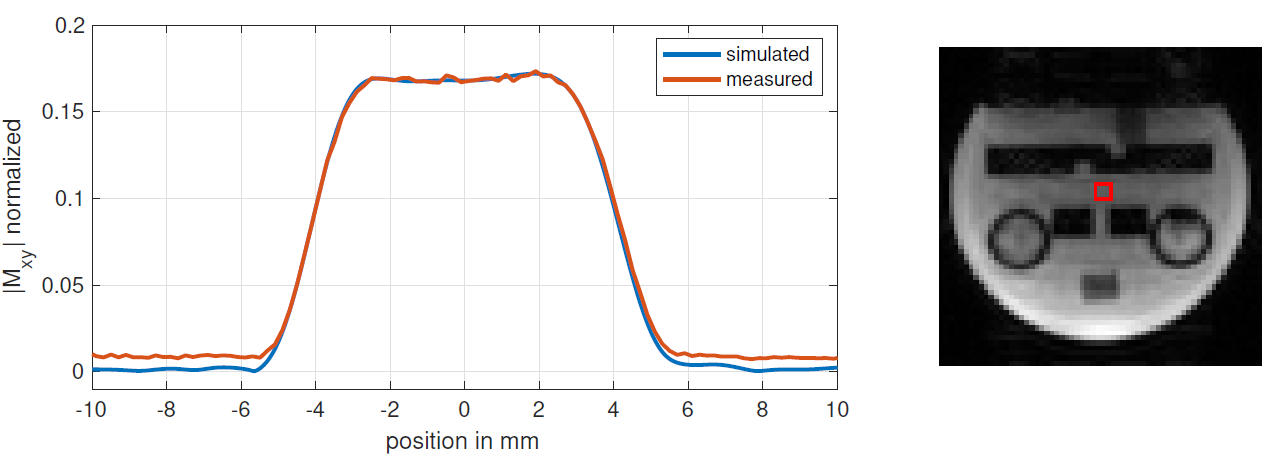
Figure 2 shows a representative deep learning (DL) prediction (library I) of an excitation not seen by the NN. The NN produces an RF pulse with a NRMSE of $$$\left( 1.57 \pm 1.11 \right)\% $$$ and a gradient of $$$\left( 0.75 \pm 0.00 \right)\% $$$ as an estimation how the predicted and the target values match. After performing an additional Bloch simulation one can identify a mismatch of the resulting magnetization profile of $$$\left( 2.38\pm 2.20 \right)\% $$$ . Figure 3 shows the NRMSE of the magnetization, of the DL predicted RF pulses (library I) and of the slice-selective gradient shapes for the defined pulse parameter range. Over this range the NN predicts RF pulses for validation data sets with a mean NRMSE of $$$\left( 1.60 \pm 1.20 \right)\% $$$ and gradients of $$$\left( 0.35 \pm 0.00 \right)\% $$$ . This leads to a mean NRMSE of $$$\left( 1.70 \pm 1.48 \right)\% $$$ for the magnetization profile. The performance declines towards the boundaries of parameter space leading to a maximum NRMSE of $$$\left( 5.67 \pm 5.17 \right)\% $$$ for a slice shift of $$$\delta z = 20\,mm$$$ due to a higher complexity of the data.
Figure 4 shows DL predicted SMS pulses using library I (SMS pulses not included) (a) and library II (SMS pulses included) (b) for training. It can be clearly seen that the DL prediction fails to design RF pulses for SMS excitations in (a) if SMS pulses were not included in the library. In this case we have a minimum NRMSE of $$$\left( 32.70 \pm 30.41 \right)\% $$$ for the predicted magnetization. Figure 4 (b), however, demonstrates that SMS pulses can also be predicted with a similar NRMSE as the prediction of single-slice pulses if they are included during training. The pulses were tested with a phantom measurement at 3T (Figure 5).

Conclusion

Comparing the results with the Bloch simulations and with measurements on a 3T system show initial promising results for the use of DL for RF pulse and gradient design. We achieved good accuracy, similar to comparable approaches. These insights serve as a basis for more complex pulses for future neural network design.

Acknowledgements

We gratefully acknowledge funding from the German Research Foundation (GRK2260, BIOQIC).

References

1) A. Rund, C. Aigner, K. Kunisch, R. Stollberger. Simultaneous multislice refocusing via time optimal control. MRM. 2018;80:1416-1428.

2) C. Aigner, A. Rund, S. Abo Seada, et al. Time optimal control‐based RF pulse design under gradient imperfections. MRM. 2020;83:561– 574.

3) D. Shin and J. Lee. DeepRF: Designing an RF pulse using a self-learning machine. ISMRM. 2020, Volume 28.

4) R. Tomi-Tricot, V. Gras, B. Thirion, et al. Smartpulse, a machine learning approach for calibration-free dynamic rf shimming: Preliminary study in a clinical environment. MRM. 2019;82:2016–2031.

5) M. S. Vinding, C. S. Aigner, S. Schmitter, et al. DeepControl: 2D RF pulses facilitating B1+ inhomogeneity and B0 off-resonance compensation in vivo at 7T. arXiv e-prints, page arXiv:2009.12408, 2020.

6) M. S. Vinding, B. Skyum, R. Sangill, et al. Ultrafast (milliseconds), multidimensional RF pulse design with deep learning. MRM.2019; 82:586–599.

7) J. Pauly, P. Le Roux, D. Nishimura, and A. Macovski. Parameter relations for the Shinnar- Le Roux selective excitation pulse design algorithm. IEEE transactions on medical imaging. 1991;10:53–65.

8) Raddi and Klose. A generalized estimate of the SLR B polynomial ripples for RF pulse generation. Journal of magnetic resonance. 1998;132:260–265.

9.) J. Shao, V. Ghodrati, K.-L. Nguyen, and P. Hu. Fast and accurate calculation of myocardial T1 and T2 values using deep learning Bloch equation simulations (DeepBLESS). Magnetic Resonance in Medicine. 2020;84(5):2831–2845.

Figures

Figure 1: (a) Network architecture for learning the RF pulse and the gradient for a given slice profile. The input layer is followed by 2 convolutional layers with a filter size of 3 and 64 total filter. The ResNet blocks are similarly constructed. Additional convolutional and 3 dense layers are added which are followed by an output layer. ReLU and SeLU are used as activation functions. (b) An example of one data set is depicted. The transversal and longitudinal magnetization act as the input data of the neural network. As the output the normalized RF pulse and the normalized gradient are used.

Figure 2: Representative example for a validation data set with a BWTP of 7, FA of 45°, slice thickness of 7mm and no slice shift used on the pretrained neural network is shown. In (e), (f), (g) the output is compared to the ground truth. The prediction is used for a second Bloch simulation to analyze the difference between the desired and the predicted magnetization in (a), (b), (c), (d). The predicted result is in good agreement with the ground truth for this parameter set.

Figure 3: The NRMSE over the whole parameters space. In blue the results for the Network I trained on 1D slice-selective SLR pulses for different validation data sets are shown. In red the same principle was extended to Network II, for which SMS pulses were included in the library. The first row ((a)-(c) displays the influence of the BWTP, the second row ((d)-(f)) with respect to the FA and the third row ((g)-(i)) to a varying slice thickness . The last row ((j)-(l)) shows the influence of the slice shift . The relations are evaluated for the magnetization profile, the RF pulse and the gradient.

Figure 4: (a) Results for DL predicted SMS using Network I with library I for training. The design of RF pulses clearly fails for SMS excitation patterns. (b) Results for DL predicted SMS using Network II, which was trained with library II containing SMS pulses. For this example, there is a good agreement between ground truth and prediction for designing SMS pulses.

Figure 5: Phantom measurement for validating the prediction of the magnetization on a 3T Siemens Magnetom Verio Scanner with a head coil. A good agreement between measured and predicted magnetization can be observed within the profile. Outside the slice profile the magnetization has non-zero values due to an increased noise level in the measurement.

Proc. Intl. Soc. Mag. Reson. Med. 29 (2021)

0230