0225
Deep Low-rank plus Sparse Network for Dynamic MR Imaging1Research Center for Medical AI, Shenzhen Institutes of Advanced Technology, Chinese Academy of Sciences, Shenzhen, China, 2Shenzhen College of Advanced Technology, University of Chinese Academy of Sciences, Shenzhen, China, 3Paul C. Lauterbur Research Center for Biomedical Imaging, Shenzhen Institutes of Advanced Technology, Chinese Academy of Sciences, Shenzhen, China
Synopsis
In dynamic MR imaging, L+S decomposition, or robust PCA equivalently, has achieved stunning performance. However, the selection of parameters of L+S is empirical, and the acceleration rate is limited, which are the common failings of iterative CS-MRI reconstruction methods. Many deep learning approaches were proposed to address these issues, but few of them used the low-rank prior. In this paper, a model-based low-rank plus sparse network, dubbed as L+S-Net, is proposed for dynamic MR reconstruction. Experiments on retrospective and prospective cardiac cine dataset show that the proposed model outperforms the state-of-the-art CS and existing deep learning methods.
Introduction
Acceleratingdynamic MRI with highly undersampled k-space has raised tremendous research
interest. Compressed sensing (CS) significantly increased the MR imaging speed and
quality with various priors. Sparse prior was well explored following a
technical path of gradually relaxing constraints. Early research used fixed
basis such as temporal Fourier transform and Wavelet transforms to sparsify
images in the x-t domain[1-4]. Then in dictionary learning and manifold
learning, the fixed basis was replaced by a learned adaptive basis from acquired
data[5-7]. Recently, deep-learning-based methods with more relaxed constraint
demonstrated great potential in fast MR imaging[8-10]. Meanwhile, low-rank
prior was introduced as an extension of sparsity in two forms: L&S [11, 12]
and L+S[13-15]. L+S decomposed the data matrix into a low-rank background component(L)
and a sparse dynamic component(S). Due to the appropriate modeling, L+S has
achieved successful applicants in lots of fields besides MR imaging, such as
foreground and background separation in computer vision[13, 16], clutter
suppressing in Ultrasound Flow imaging[17] and image alignment[18]. However,
the low-rank prior brings more parameters to tune in the reconstruction, which exacerbated
the empirical selection of the regularization parameters in CS methods.
Besides, the singular value decomposition performed at each iteration is time
consuming. Our work focuses on dealing with these problems by unrolling L+S
into a deep network.
Methods
Thereconstruction model in this paper can be considered as follow:
$$\min_{\boldsymbol{L,S,X}}\|\boldsymbol{AX-y}\|_2^2+\lambda_L\|\boldsymbol{L}\|_*+\lambda_S\| \boldsymbol{DS}\|_1,\quad s.t.\boldsymbol{X=L+S}\qquad\qquad\qquad (1)$$
Problem
(1) can be solved via a linearized alternating minimization method and get the
following iterative steps:
$$\left\{\begin{align*}\boldsymbol{L}_{k+1}&=\boldsymbol{H}_{\lambda_L}(\boldsymbol{X}_k-\boldsymbol{S}_k)\\\boldsymbol{S}_{k+1}&=\boldsymbol{P}_{\lambda_S}(\boldsymbol{X}_k,\boldsymbol{L}_{k+1})\\\boldsymbol{X}_{k+1}&=\boldsymbol{L}_{k+1}+\boldsymbol{S}_{k+1}\gamma\nabla\boldsymbol{F}(\boldsymbol{L}_{k+1}+\boldsymbol{S}_{k+1})\end{align*}\right.\qquad\qquad\qquad (2)$$
where
$$\boldsymbol{H}_\lambda(\boldsymbol{X})=\boldsymbol{U}\boldsymbol{\Lambda}_\lambda(\Sigma)\boldsymbol{V}^*\qquad\qquad\qquad (3)$$
is
singular value thresholding (SVT) operator, $$$\boldsymbol{X}=\boldsymbol{U}\boldsymbol{\Sigma}\boldsymbol{V}^*$$$ is the singular
value decomposition of $$$\boldsymbol{X}$$$. $$$\boldsymbol{\Lambda}$$$ is the soft thresholding operator as follow:
$$\boldsymbol{\Lambda}_\lambda(x)=\frac{x}{|x|}\max(|x|=\lambda,0)\qquad\qquad\qquad (4)$$
In
Eq.(2), $$$\boldsymbol{P}_\lambda(\cdot)$$$ is a proximal operator depending on
the sparse transform $$$\boldsymbol{D}$$$. $$$\gamma$$$ is the update step size.
There
are three intractable problems. First, because the proximal operator $$$\boldsymbol{P}_\lambda(\cdot)$$$ is achieved via proximal gradient method, the
closed form can only be achieved when the transform matrix $$$\boldsymbol{D}$$$ is orthogonal (for
example, temporal FFT). If a fixed orthogonal transform is adopted, the sparse
representation will be limited. Second, the selection of the parameters $$$\lambda_L,\lambda_S,\gamma$$$ is empirical. Third, the iteration algorithms
usually take many steps before converging, which makes the reconstruction time
very long.
The
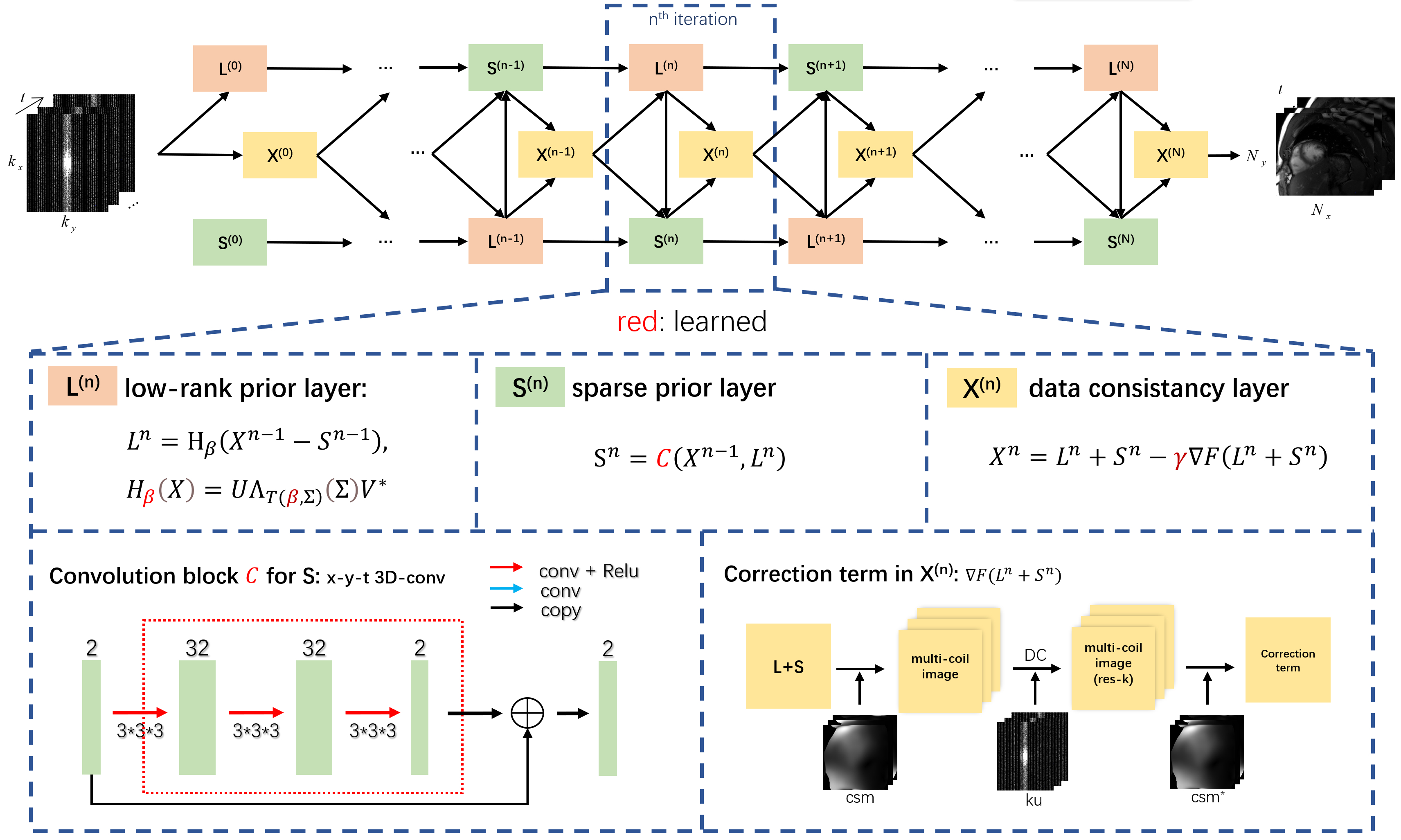
unrolling low-rank plus sparse network (L+S-Net) tackles all the problems well.
The iteration steps are unrolled into several iteration blocks. As shown in
Fig.1, each of the blocks contains three network modules, which are named as
low-rank prior layer $$$\boldsymbol{L}^k$$$, sparse prior
layer $$$\boldsymbol{S}^k$$$ and data consistency
layer $$$\boldsymbol{X}^k$$$ corresponding to the update steps in Eq.(2):
$$\left\{\begin{align*}\boldsymbol{L}^{k+1}:&\ \boldsymbol{L}_{k+1}=\boldsymbol{H}_{\lambda_L}(\boldsymbol{X}_k-\boldsymbol{S}_k)\\\boldsymbol{S}^{k+1}:&\ \boldsymbol{S}_{k+1}=\boldsymbol{P}_{\lambda_S}(\boldsymbol{X}_k,\boldsymbol{L}_{k+1})\\\boldsymbol{X}^{k+1}:&\ \boldsymbol{X}_{k+1}=\boldsymbol{L}_{k+1}+\boldsymbol{S}_{k+1}\gamma\nabla\boldsymbol{F}(\boldsymbol{L}_{k+1}+\boldsymbol{S}_{k+1})\end{align*}\right.\qquad\qquad\qquad (5)$$
where $$$\boldsymbol{H}_\beta$$$ is a learned
SVT operator, which shares the same calculation process with the traditional
SVT, but the threshold $$$\lambda_L$$$ is replaced with a learnable $$$T(\beta,\boldsymbol{\Sigma})$$$
$$T(\beta,\boldsymbol{\Sigma})=Sigmoid(\beta)*\sigma_1\qquad\qquad\qquad (6)$$
where $$$\sigma_1$$$ is the maximal singular value in $$$\boldsymbol{\Sigma}$$$. The proximal operator $$$\boldsymbol{P}_{\lambda_S}$$$ is also replaced with a CNN $$$\boldsymbol{C}$$$ to achieve better performance.
Experiment
Thefully sampled cardiac cine data were collected from 29 healthy volunteers on a
3T scanner (MAGNETOM Trio, Siemens Healthcare, Erlangen, Germany) with a
20-channel receiver coil array. The following sequence parameters were used:
FOV = 330*330 mm, acquisition matrix = 256*256, slice thickness = 6 mm, and
TR/TE = 3.0 ms/1.5 ms. the coil sensitivity maps were calculated from the
undersampled time-averaged k-space using ESPIRiT algorithm. We obtained 800 2D-t cardiac MR data for
training and 118 data for testing after data augmentation. The models was implemented
on an Ubuntu 16.04 LTS (64-bit) operating system equipped with an Intel Xeon
E5-2640 CPU and a Tesla TITAN Xp GPU. The open framework TensorFlow was used.
Results
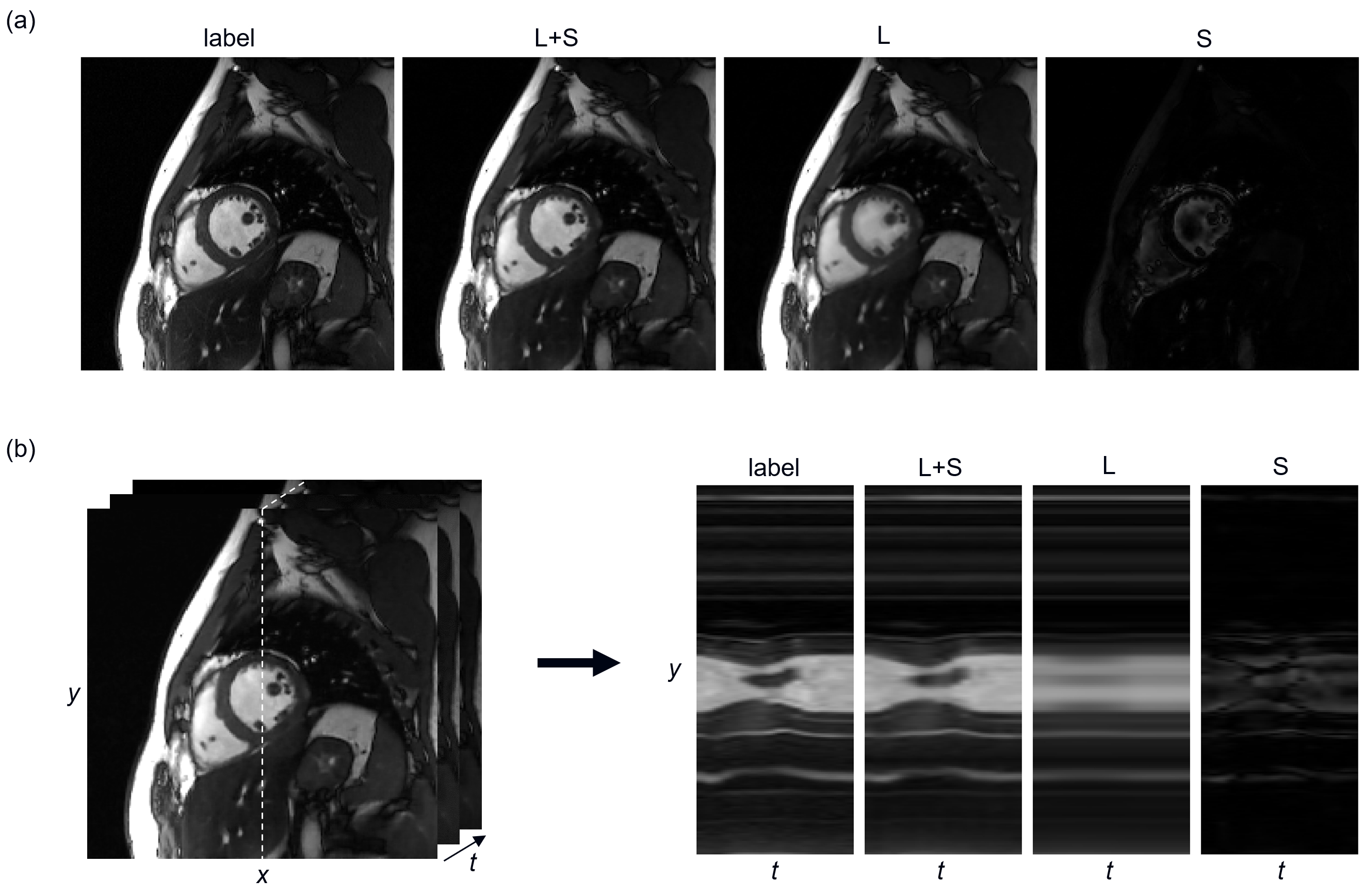
Fig.2 shows the separation of L andS components at 8-fold acceleration, which meets the hypothesis of low-rank
plus sparse. From the y-t view, we can clearly observe that the L component is
a slowly changing background rather than a static one. The low-rank property
holds well in the test dataset. The S component is already sparse without a sparse
transform.
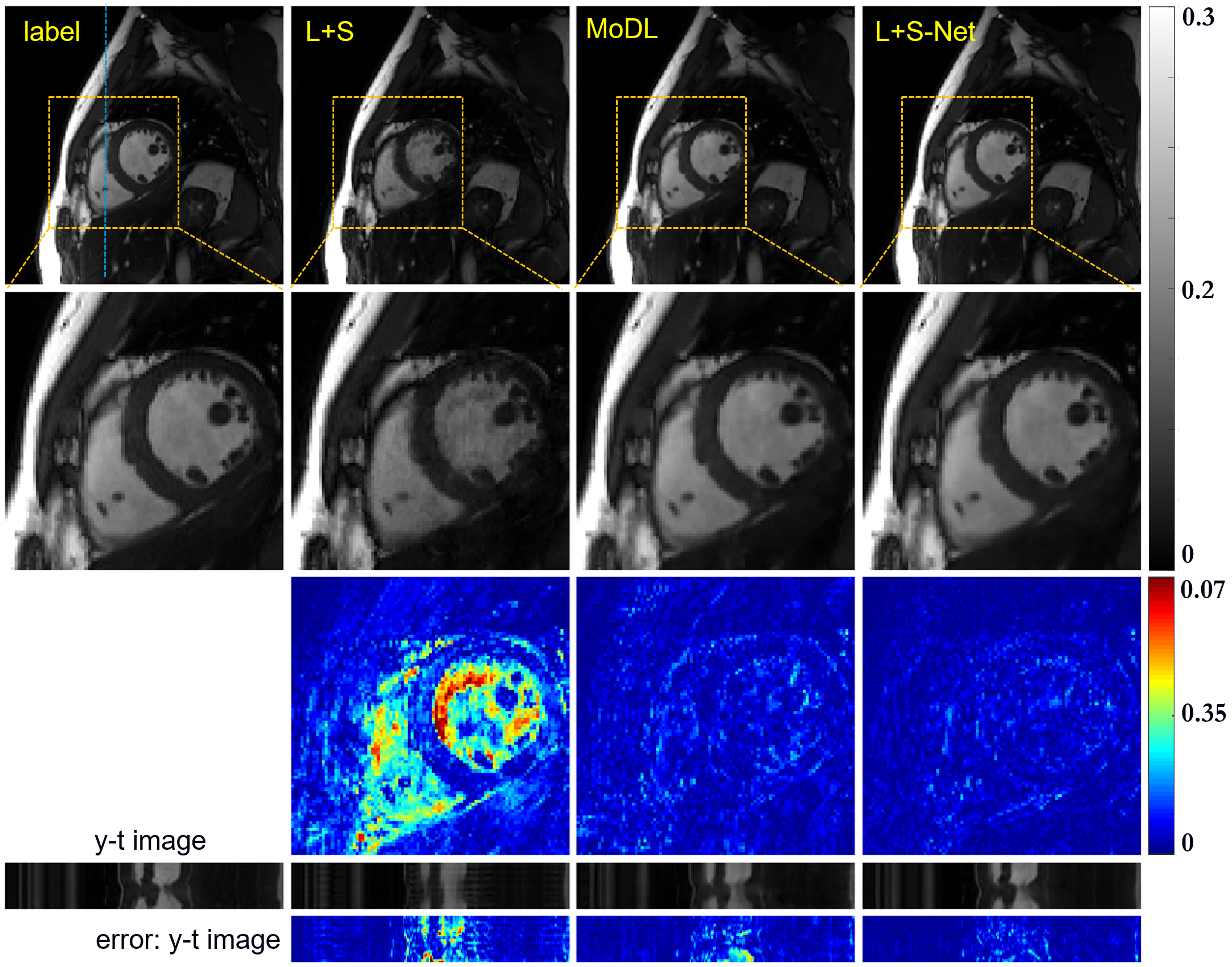
Fig.3 shows the comparison between
the results of L+S, MoDL, and the proposed L+S-Net at 12-fold acceleration. L+S
almost failed at such a high acceleration rate, the reconstruction result of
which shows a lot of artifacts. The MoDL method achieved acceptable results. We
can see the proposed L+S-Net performs better, especially from the error map.
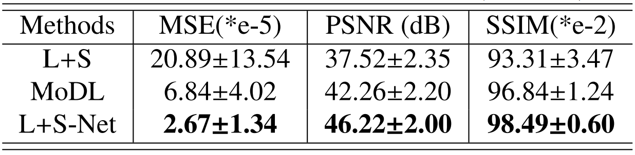
The quantitative results in Table.1 correspond to the visual comparison.
Conclusion
In this paper, we propose amodel-based unrolled low-rank plus sparse network, dubbed as L+S-Net, for
dynamic MR reconstruction. A learned singular value thresholding was introduced
to explore deep low rank prior in dynamic images. Experiment results show that
our method can improve the reconstruction result both qualitatively and
quantitatively.
Acknowledgements
This work was supported in part by the National Key R&D Program of China (2017YFC0108802 and 2017YFC0112903); National Natural Science Foundation of China (61771463, 81830056, U1805261, 81971611, 61871373, 81729003, 81901736); Natural Science Foundation of Guangdong Province (2018A0303130132); Key Laboratory for Magnetic Resonance and Multimodality Imaging of Guangdong Province; Shenzhen Peacock Plan Team Program (KQTD20180413181834876); Innovation and Technology Commission of the government of Hong Kong SAR (MRP/001/18X); Strategic Priority Research Program of Chinese Academy of Sciences (XDB25000000).References
1. Donoho D L. Compressed sensing[J]. IEEE Transactions on information theory, 2006, 52(4): 1289-1306.
2. Lustig M, Donoho D, Pauly J M. Sparse MRI: The application of compressed sensing for rapid MR imaging[J]. Magnetic Resonance in Medicine: An Official Journal of the International Society for Magnetic Resonance in Medicine, 2007, 58(6): 1182-1195.
3. Otazo R, Kim D, Axel L, et al. Combination of compressed sensing and parallel imaging for highly accelerated first‐pass cardiac perfusion MRI[J]. Magnetic resonance in medicine, 2010, 64(3): 767-776.
4. Ma S, Yin W, Zhang Y, et al. An efficient algorithm for compressed MR imaging using total variation and wavelets[C]//2008 IEEE Conference on Computer Vision and Pattern Recognition. IEEE, 2008: 1-8.
5. Wang Y, Ying L. Compressed sensing dynamic cardiac cine MRI using learned spatiotemporal dictionary[J]. IEEE transactions on Biomedical Engineering, 2013, 61(4): 1109-1120.
6. Caballero J, Price A N, Rueckert D, et al. Dictionary learning and time sparsity for dynamic MR data reconstruction[J]. IEEE transactions on medical imaging, 2014, 33(4): 979-994.
7. Nakarmi U, Wang Y, Lyu J, et al. Dynamic magnetic resonance imaging using compressed sensing with self-learned nonlinear dictionary (NL-D)[C]//2015 IEEE 12th International Symposium on Biomedical Imaging (ISBI). IEEE, 2015: 331-334.
8. Schlemper J, Caballero J, Hajnal J V, et al. A deep cascade of convolutional neural networks for dynamic MR image reconstruction[J]. IEEE transactions on Medical Imaging, 2017, 37(2): 491-503.
9. Qin C, Schlemper J, Caballero J, et al. Convolutional recurrent neural networks for dynamic MR image reconstruction[J]. IEEE transactions on medical imaging, 2018, 38(1): 280-290.
10. Wang S, Ke Z, Cheng H, et al. DIMENSION: Dynamic MR imaging with both k‐space and spatial prior knowledge obtained via multi‐supervised network training[J]. NMR in Biomedicine, 2019: e4131.
11. Lingala S G, Hu Y, DiBella E, et al. Accelerated dynamic MRI exploiting sparsity and low-rank structure: kt SLR[J]. IEEE transactions on medical imaging, 2011, 30(5): 1042-1054.
12. Zhao B, Haldar J P, Christodoulou A G, et al. Image reconstruction from highly undersampled (k, t)-space data with joint partial separability and sparsity constraints[J]. IEEE transactions on medical imaging, 2012, 31(9): 1809-1820.
13. Candès E J, Li X, Ma Y, et al. Robust principal component analysis?[J]. Journal of the ACM (JACM), 2011, 58(3): 1-37.
14. Chandrasekaran V, Sanghavi S, Parrilo P A, et al. Rank-sparsity incoherence for matrix decomposition[J]. SIAM Journal on Optimization, 2011, 21(2): 572-596.
15. Otazo R, Candes E, Sodickson D K. Low‐rank plus sparse matrix decomposition for accelerated dynamic MRI with separation of background and dynamic components[J]. Magnetic resonance in medicine, 2015, 73(3): 1125-1136.
16. Mansour H, Vetro A. Video background subtraction using semi-supervised robust matrix completion[C]//2014 IEEE International Conference on Acoustics, Speech and Signal Processing (ICASSP). IEEE, 2014: 6528-6532.
17. Ashikuzzaman M, Belasso C, Kibria M G, et al. Low rank and sparse decomposition of ultrasound color flow images for suppressing clutter in real-time[J]. IEEE transactions on medical imaging, 2019, 39(4): 1073-1084.
18. Peng Y, Ganesh A, Wright J, et al. RASL: Robust alignment by sparse and low-rank decomposition for linearly correlated images[J]. IEEE transactions on pattern analysis and machine intelligence, 2012, 34(11): 2233-2246.
Figures