0173
Optimized multi-axis spiral projection MRF with subspace reconstruction for rapid 1-mm isotropic whole-brain MRF in 2 minutes1Department of Rdiology, Stanford university, Stanford, CA, United States, 2Department of Electrical Engineering, Stanford university, Stanford, CA, United States, 3Athinoula A. Martinos Center for Biomedical Imaging, Massachusetts General Hospital, Charlestown, MA, United States, 4Department of Electrical Engineering and Computer Science, MIT, Cambridge, MA, United States, 5Center for Brain Imaging Science and Technology, Department of Biomedical Engineering, Zhejiang University, Hangzhou, China, 6Department of Imaging Sciences, University of Rochester, Rochester, NY, United States, 7Department of Radiology, Harvard Medical School, Cambridge, MA, United States
Synopsis
To improve the quality and speed of 3D MRF, we applied spatiotemporal subspace reconstruction to 3D MRF and further modified its spiral-projection spatiotemporal encoding scheme. When compared to conventional sliding-window iNUFFT reconstruction, the subspace reconstruction provided markedly improved quantitative maps, with lower artifacts and higher SNR. The optimized spiral-projection encoding scheme, which was designed to increase spatiotemporal incoherency, was also validated to be more robust to artifacts, particularly at high accelerations. The proposed method enables high-quality whole-brain T1, T2, and proton density mapping with 1-mm isotropic resolution in 2 minutes and 0.8-mm isotropic resolution in ~4minutes.
Introduction
Magnetic Resonance Fingerprinting (MRF)1 is a fast quantitative imaging technique for estimating multiple tissue parameters simultaneously. Several 3D high-resolution MRF techniques2-5 have been developed to improve the image quality of MRF. Our previous work6 proposed a 3D MRF technique which could achieve whole-brain 1-mm isotropic resolution within 6 minutes based on multi-axis spiral-projection trajectory and sliding-window iNUFFT reconstruction7. Building on this work, we applied spatiotemporal subspace reconstruction8,9 and optimize its spiral-projection spatiotemporal encoding to achieve better image quality and higher acceleration.Method
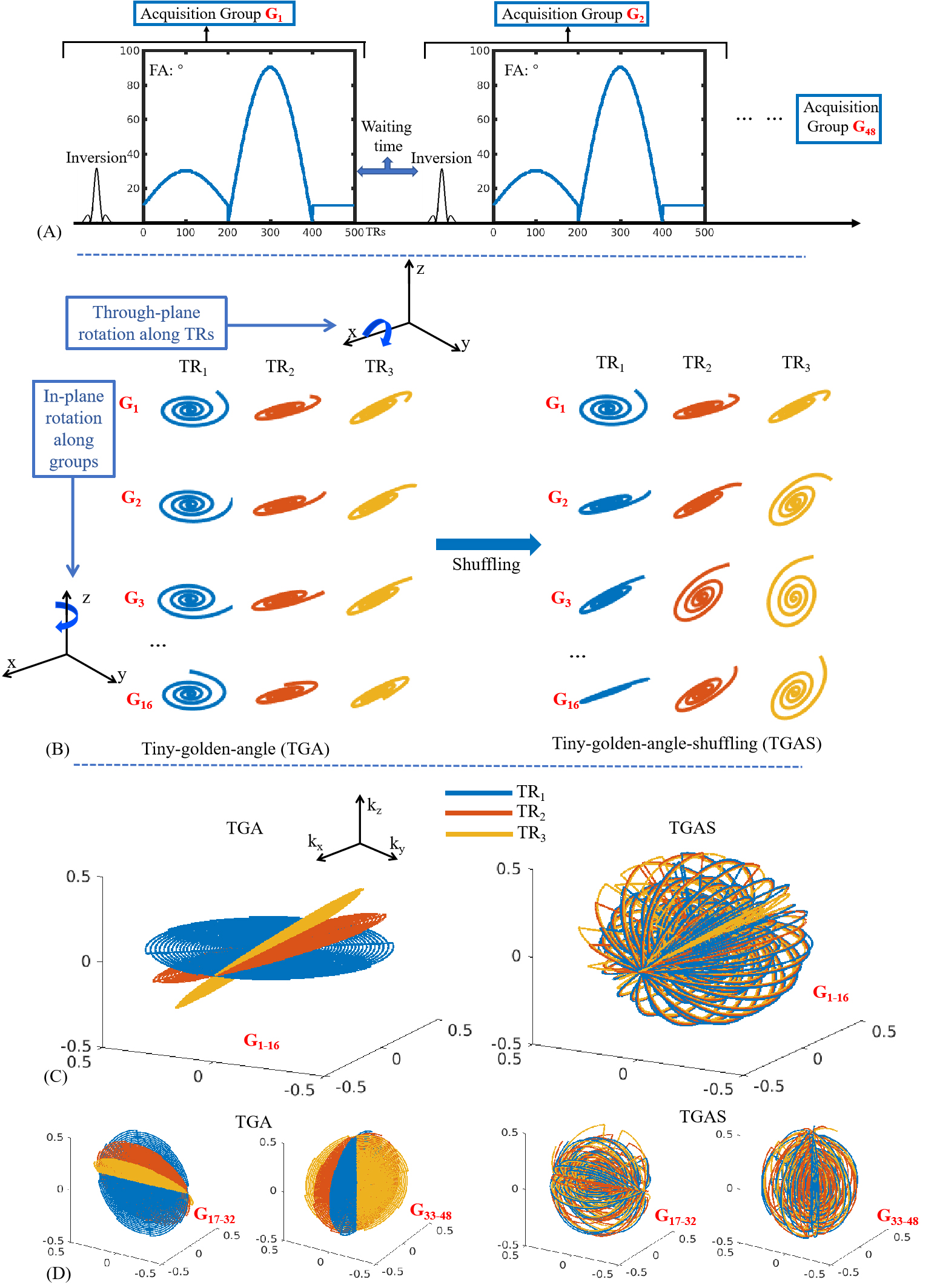
Sequence: Fig1A shows the SPI-MRF FISP sequence diagram where data are acquired across 500 TRs per acquisition group, with multiple groups performed sequentially to achieve adequate 3D k-space encoding. Each acquisition group contains an adiabatic inversion preparation with TI=20ms, follows by variable-FA acquisitions where the TR=12ms and TE=1.8ms. A waiting time of 1.2s was left to allow relaxation for better SNR, resulting in a net acquisition per group of 7.2s.Fig1B shows the spiral-projection k-space encoding across TRs and acquisition groups for two different encoding schemes: i) tiny-golden-angle(TGA) and ii) tiny-golden-angle-shuffling(TGAS). In our previous work, the TGA scheme (Fig1B-left) was used with sliding-window reconstruction to achieve good performance. As an example, for a 1-mm isotropic acquisition across a FOV of 220×220×220mm3, 48 acquisition groups are obtained in a total acquisition time of 5m46s(refer to as R=1 acquisition). Here, a variable density spiral with 16× acceleration at the center and 32× at the edge of k-space is used. For the first 16 acquisition groups(G1-16) in TGA, in-plane rotation(z-axis) was implemented along the acquisition group dimension to obtain the full 16 spiral interleaves, while through-plane rotation(x-axis) was performed along the TR-dimension using tiny golden angle10 of 23.63° as shown in Fig1C-left; i.e. $$${\it Θ}_{x}(j)=23.63°×j,{\it θ}_{z}(i)=22.5°×i$$$ where j is the TR index and i is the group index. To achieve multi-axis rotation, groups G17-32 and G33-48 were designed to rotate along x- and y-axis for in-plane rotation and y- and z-axis for through-plane rotation, respectively (Fig1D-left).
In this work, we propose the TGAS spatiotemporal scheme which shuffles the rotation operation via: $$${\it Θ}_{x}(i,j)=23.63°×(i+j),{\it θ}_{z}(i)=22.5°×i$$$ as illustrated in Fig1C&D. This increases the level of spatiotemporal incoherency, which should aid the subspace reconstruction11.
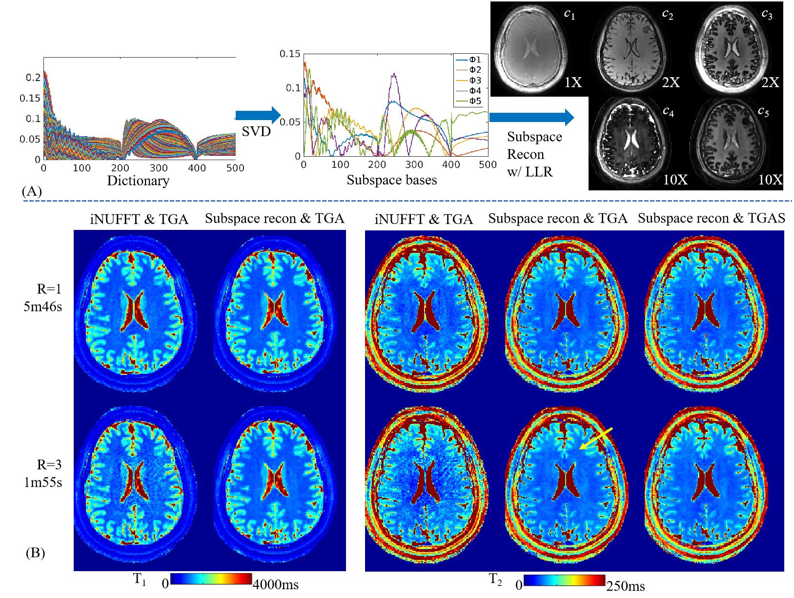
Reconstruction: Fig2A shows the process of the MRF subspace reconstruction9, where dictionary was pre-calculated using EPG12 and the first five temporal principal components extracted as subspace bases(Φ1-5). The coefficient maps(c1-5) are then calculated via:
$$\begin{array}{c}min\\c\end{array}{\parallel}PFSΦc-y{\parallel}_2^2+λR_{r}(c)$$
where P is the undersampling pattern, F is the non-uniform Fourier transform, S is the coil sensitivity, λ is the regularization parameter for locally low rank (LLR) regularization11,13 Rr(c). The sensitivity maps were estimated by ESPIRiT method14 using central k-space from all acquired TRs and groups as input. The reconstruction was performed using the BART toolbox15. Subsequent to the subspace reconstruction, the coefficient maps were used to generate MRF time-series images and the dictionary template matching applied to obtain quantitative maps.
Validation: SPI-MRF were acquired on a Siemens 3T Prisma scanner using a 32-channel head coil. 1-mm isotropic data were acquired at different acceleration factors ranging from R=2 to R=6, where undersampling was performed across the group dimension.
An additional dataset at 0.8-mm isotropic resolution was also acquired, to access the method’s capability for submillimeter quantitative mapping. To maintain the same spiral readout duration of 6.7ms as in the 1-mm case, 24 instead of 16 VDS spiral interleaves are employed, with 24×/48× acceleration at the center/edge of k-space, resulting in 72 acquisition groups (acquisition time of 8m38s for R=1). Based on SNR consideration, R=2(4m19s) was selected for used in the final 0.8-mm acquisition.
Results
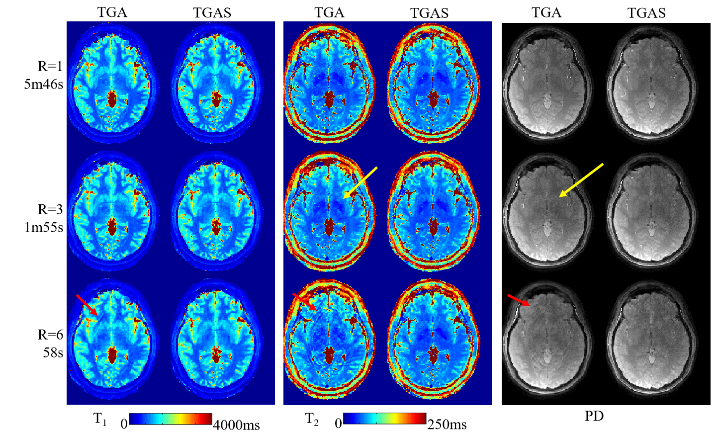
Fig2B shows comparison between sliding-window iNUFFT and subspace reconstructions, where T1&T2 maps from the subspace reconstruction of the TGA data at R=3 is of higher quality than ones from iNUFFT at R=1. There is a slight artifact indicated by the yellow arrow for TGA at R=3, which is not present in the equivalent TGAS acquisition.Fig3 further compares the performance of TGA and TGAS, both with subspace reconstruction, at various acceleration factors. The results from TGA shows slight artifacts at R=3(yellow arrows) and strong artifacts at R=6(red arrows) while the results of TGAS remain artifact-free.
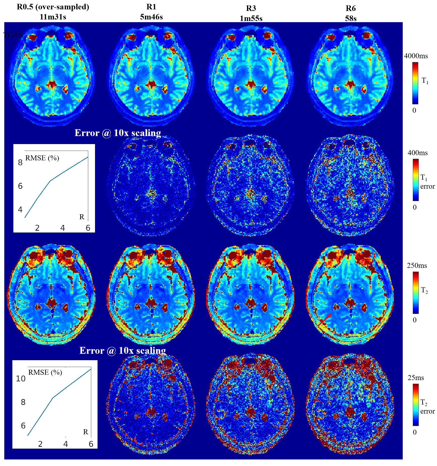
To validate the performance of TGAS, a R=0.5 dataset with high-SNR were acquired as a gold standard reference. Errors in T1&T2 maps at different acceleration factors were calculated against this gold standard data and shown in Fig4. Here, the proposed subspace reconstruction with TGAS shows good performance, achieved at R=3 with RMSE of 6.42% and 8.37%(CSF & skull excluded), while reconstruction quality remains reasonable at R=6.
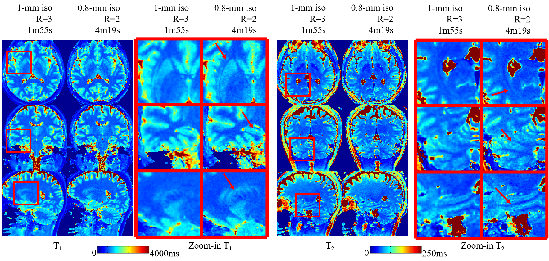
Fig5 shows that the increased resolution of the 0.8-mm isotropic acquisition can help better visualize subtle brain structures, where the zoom-ins highlight details in several specific regions.
Discussion and Conclusion
In this work, we applied a subspace reconstruction and optimized spiral-projection trajectory to improve the image quality and acquisition speed of 3D MRF. By projecting images from time domain to low-dimension subspace domain and applying LLR regularization, the reconstruction conditioning was significantly improved as well as SNR, which enables higher accelerations. An optimized shuffled 3D spiral-projection trajectory with improved spatiotemporal incoherence further improves the quantitative maps at high acceleration factors.Acknowledgements
This work was supported in part by NIH research grants: R01-EB020613, R01-EB019437, R01-MH116173, P41EB030006, and U01-EB025162.References
1. Ma, D. et al. Magnetic resonance fingerprinting. Nature 495, 187–192 (2013).
2. Liao, C. et al. 3D MR fingerprinting with accelerated stack-of-spirals and hybrid sliding-window and GRAPPA reconstruction. Neuroimage 162, 13–22 (2017).
3. Ma, D. et al. Fast 3D magnetic resonance fingerprinting for a whole-brain coverage. Magn. Reson. Med. 79, 2190–2197 (2018).
4. Gómez, P. A. et al. Rapid three-dimensional multiparametric MRI with quantitative transient-state imaging. Scientific Reports vol. 10 (2020).
5. Chen, Y. et al. High-resolution 3D MR Fingerprinting using parallel imaging and deep learning. Neuroimage 206, (2020).
6. Cao, X. et al. Fast 3D brain MR fingerprinting based on multi-axis spiral projection trajectory. Magn. Reson. Med. 82, 289–301 (2019).
7. Cao, X. et al. Robust sliding-window reconstruction for Accelerating the acquisition of MR fingerprinting. Magn. Reson. Med. 78, 1579–1588 (2017).
8. Liang, Z.-P. SPATIOTEMPORAL IMAGING WITH PARTIALLY SEPARABLE FUNCTIONS Zhi-Pei Liang Department of Electrical and Computer Engineering , and Beckman Institute for Advanced Science and Technology University of Illinois at Urbana-Champaign. IEEE Int. Symp. Biomed. Imaging 2, 988–991 (2007).
9. Zhao, B. et al. Improved magnetic resonance fingerprinting reconstruction with low-rank and subspace modeling. Magn. Reson. Med. 79, 933–942 (2018).
10. Wundrak, S. et al. Golden ratio sparse MRI using tiny golden angles. Magn. Reson. Med. 75, 2372–2378 (2016).
11. Tamir, J. I. et al. T2 shuffling: Sharp, multicontrast, volumetric fast spin-echo imaging. Magn. Reson. Med. 77, 180–195 (2017).
12. Weigel, M. Extended phase graphs: Dephasing, RF pulses, and echoes - Pure and simple. J. Magn. Reson. Imaging 41, 266–295 (2015).
13. Zhang, T., Pauly, J. M. & Levesque, I. R. Accelerating parameter mapping with a locally low rank constraint. Magn. Reson. Med. 73, 655–661 (2015).
14. Uecker, M. et al. ESPIRiT - An eigenvalue approach to autocalibrating parallel MRI: Where SENSE meets GRAPPA. Magn. Reson. Med. 71, 990–1001 (2014).
15. Uecker, M., Tamir, J. I., Ong, F. & Lustig, M. The BART Toolbox for Computational Magnetic Resonance Imaging. Ismrm (2016).
Figures