Introduction

Magnetic Resonance Fingerprinting (MRF) is a relatively new framework for quantitative MR imaging^1-4. However, the inherently long acquisition time poses challenges for improving spatial resolution, which is beneficial to detecting smaller structures and fine lesions. We designed a spiral sampling trajectory to achieve 0.8 mm isotropic resolution with the help of a novel deep learning method for effective reconstruction from undersampled data in both k-space and image space. Our preliminary results show that a total of 16x acceleration (4x in k-space and 4x in image space) can be achieved, reducing the data acquisition time for whole-brain coverage at 0.8-mm isotropic resolution to less than 5 mins.

Methods

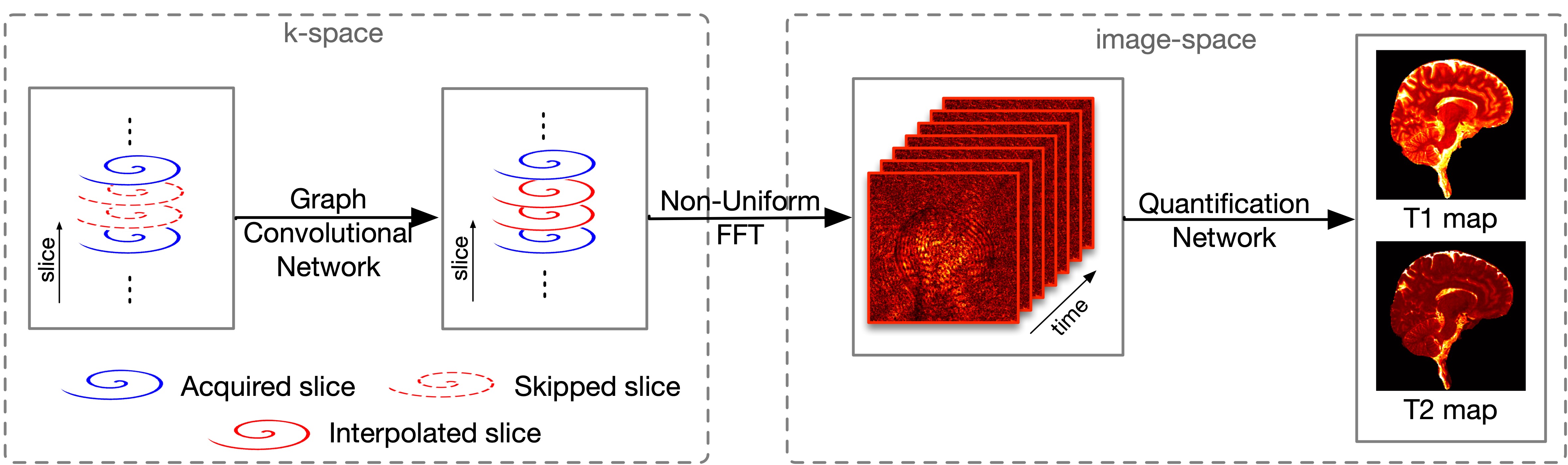
The 3D MRF data was acquired using a Siemens 3T scanner with a 32-channel receive coil. The pulse sequence was based on a stack-of-spirals trajectory with steady-state free precession (SSFP) readout. Imaging parameters: FOV, 25x25 cm; matrix size, 320x320; TR, 12.6 ms; TE, 1.3 ms; flip angles, 5-12 degrees, number of slices, 120. Acquiring a total of 768 MRF time frames required ~20 min with 2x interleaved undersampling in k-space. The gold standard is obtained using GRAPPA+template matching with the acquired data. Data were acquired for 5 subjects; 3 were used for training and 2 for testing. Retrospective data undersampling was used for numerical evaluation. Additionally, one prospectively undersampled scan with whole-brain coverage (14 cm) was acquired from one testing subject to evaluate method feasibility.
The data are undersampled by 1) interleaved undersampling along the partition-encoding direction in k-space as described in ⁴ and 2) only taking the early time frames in image space. Our method (Fig. 1) consists of 1) a Graph Convolutional Network (GCN) for interpolation of missing k-space data with acceleration factor higher than conventional parallel imaging ⁷ and 2) a Quantification Network for robust tissue property mapping using data subsampled in the temporal dimension ⁶. Non-uniform FFT is applied to convert the reconstructed k-space data to image space.
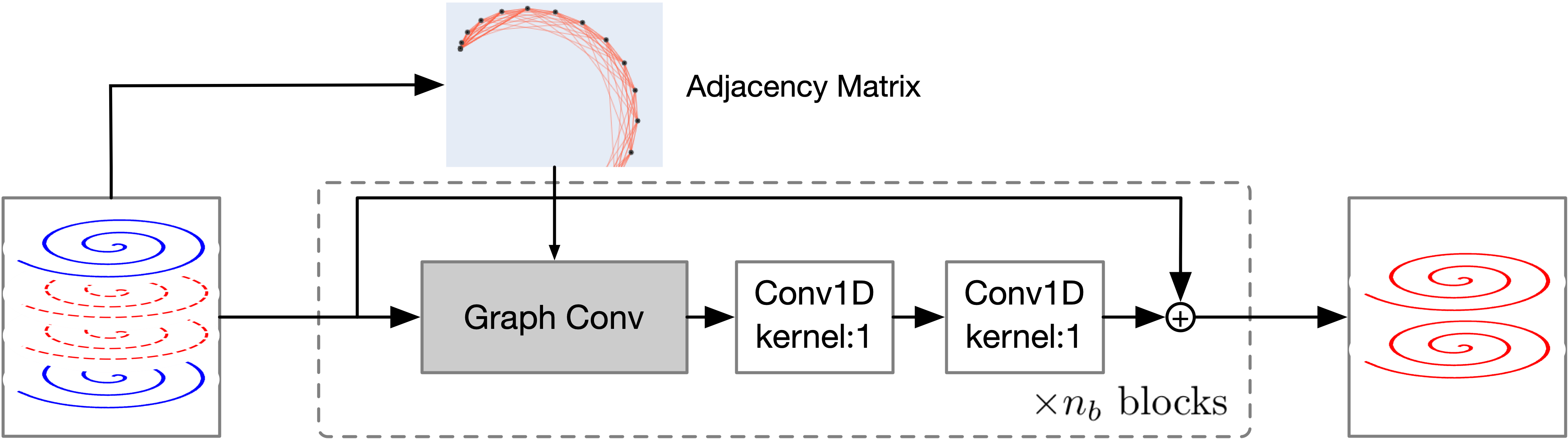
The GCN (Fig. 2) consists of $$$n_b$$$ blocks and each block is constructed with one graph convolutional layer⁵ with kernel size 5 and two 1D-Convolution layers with kernel size 1. The output of each block is added to the output of the next block. All the layers are ReLU activated, with the exception of the last layer, which is linearly activated. The number of filters of the three convolutional layers in each block are 512, 1024, and 1024. In each block, the graph convolutional layer aggregates information from spatial neighbors in k-space and the subsequent two convolution layers map the data to a high-dimension space to learn the relationships between data points. The residual connections ease training convergence and reduce error propagation. The GCN is trained based on the k-space data containing the central 16 partitions to cater to undersampling with factor 4 along the partition-encoding direction.
The quantification network ⁶ consists of a Fully Convolutional Network (FCN) and a U-Net. The FCN is composed of 3 kernel-1 convolutional layers with 64 filters. The U-Net consists of 3 down-sample blocks and 3 up-sample blocks with 64 initial filters. For acceleration, only the first 192 time points (25%) is used. The reference high-quality T1 and T2 maps are obtained from all 768 time points without acceleration along the partition-encoding direction.

Results

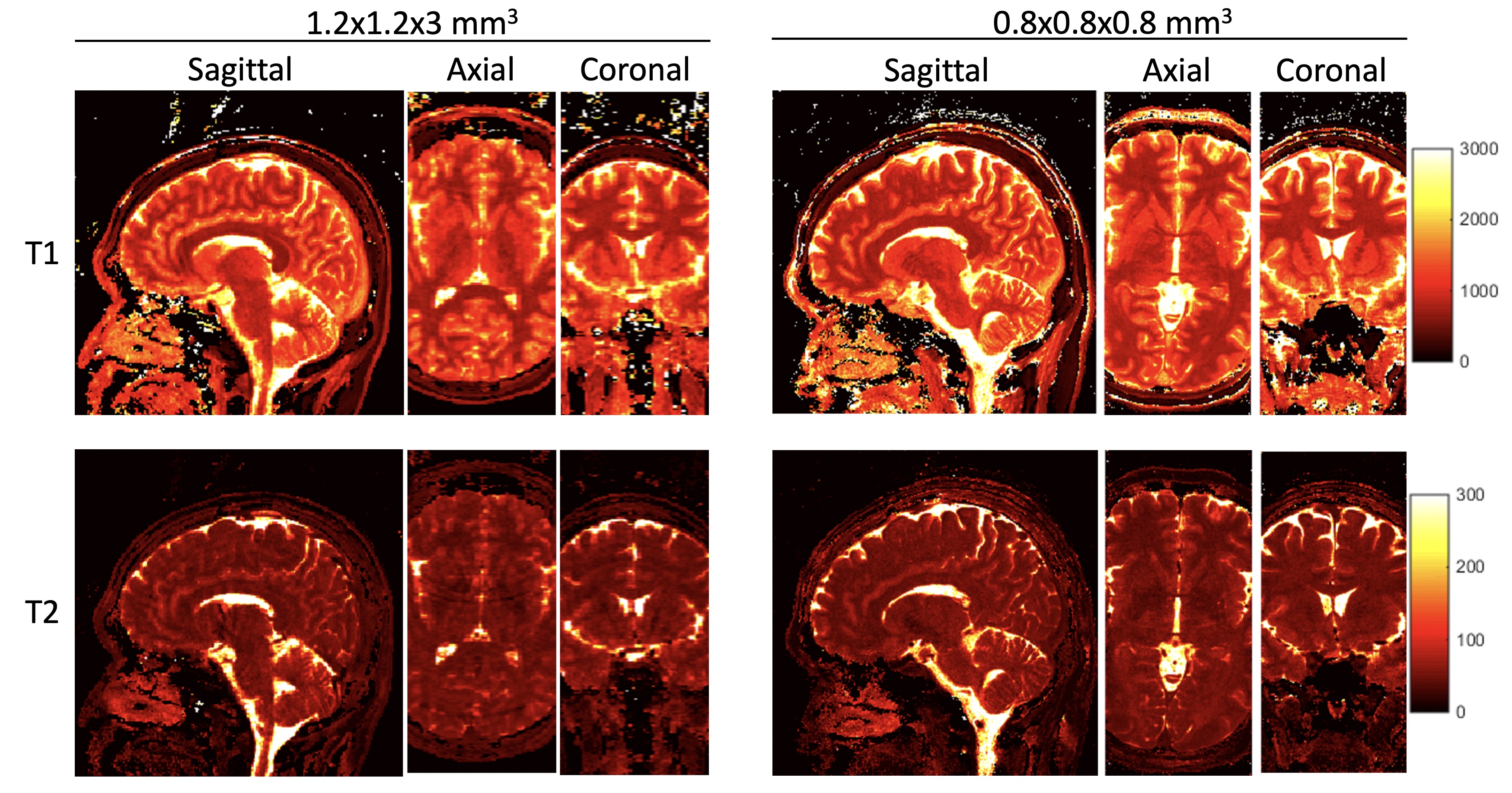
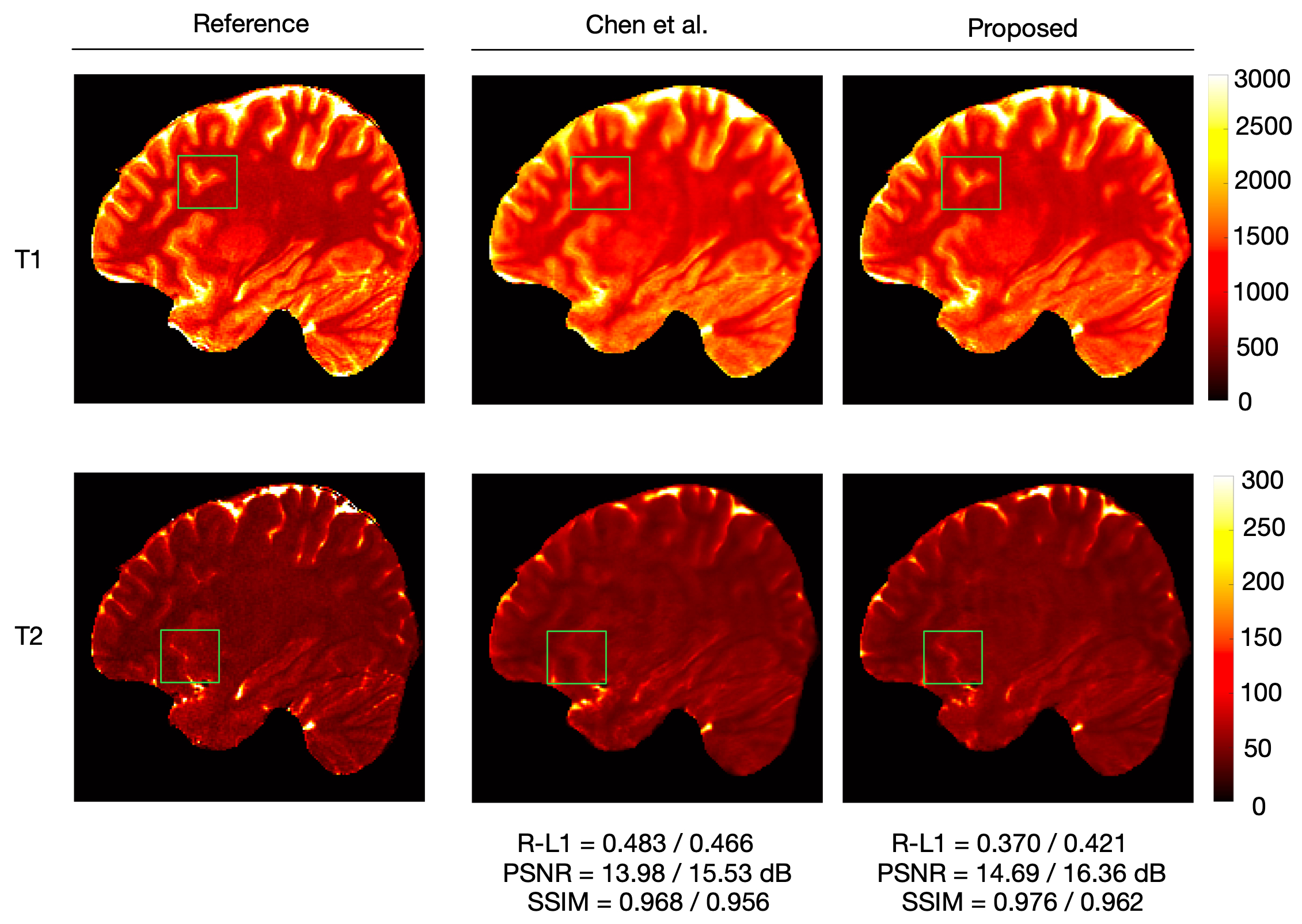
Fig. 3 shows representative T1 and T2 maps obtained using 3D MRF with both 1.2x1.2x3 mm³ and 0.8 mm isotropic resolutions from the same subject, demonstrating the superior details in high-resolution MRF.
Fig. 4 shows representative T1 and T2 maps generated from the MRF data acquired with 16x acceleration. Compared with prior methods ^4,7, the proposed method yields improvements as indicated by the qualitative maps and the quantitative metrics (average Relative-L1, PSNR, and SSIM).
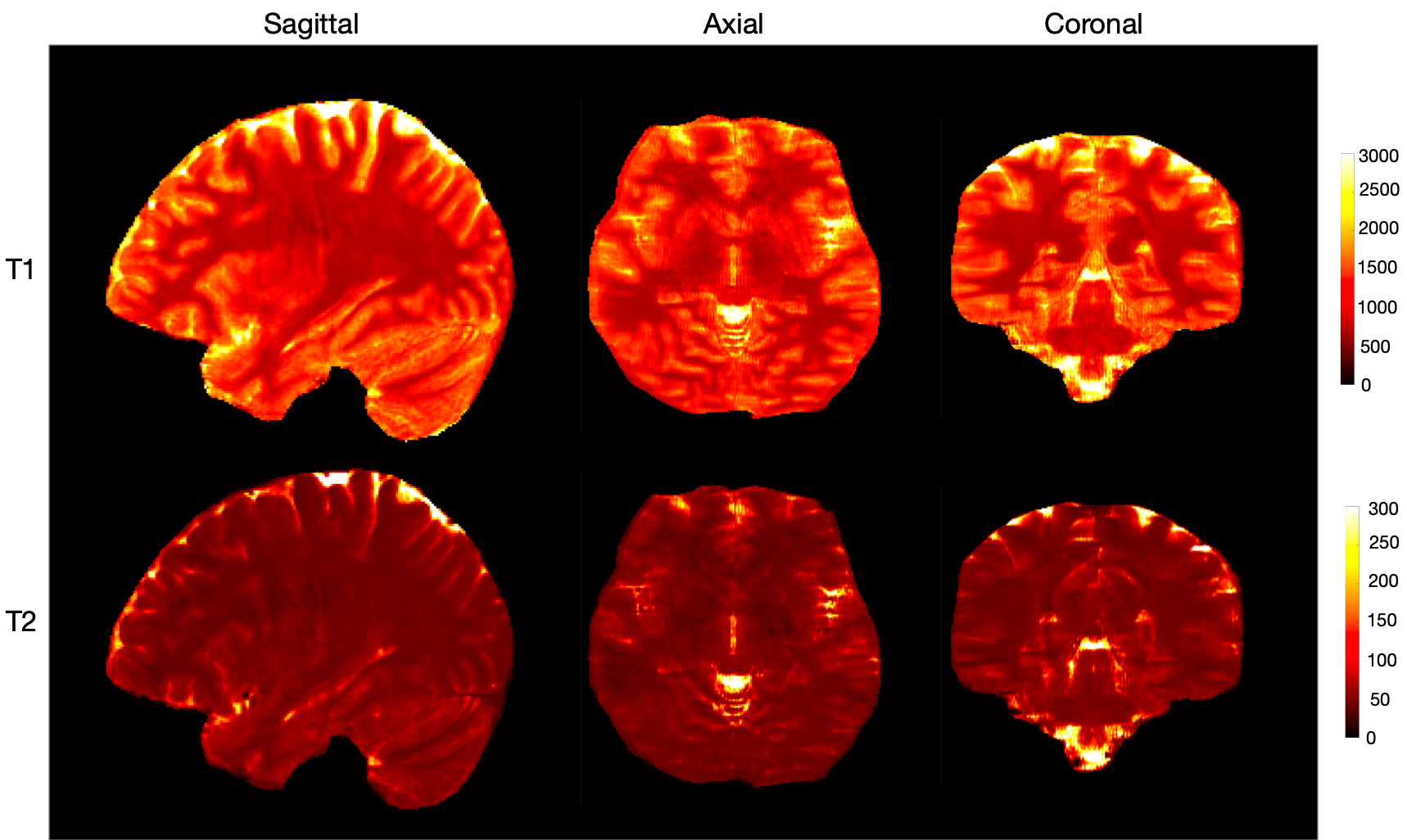
Fig. 5 shows whole-brain quantitative T1 and T2 maps obtained from the prospectively undersampled data in three views. Blurriness in the axial and coronal views is expected to decrease with training using more samples.

Discussion and Conclusion

We developed a novel deep learning method to accelerate submillimeter 3D MRF, improving the feasibility of high-resolution quantitative mapping in clinical settings. We expect further improvement in tissue quantification accuracy with training using a larger sample size.

Acknowledgements

This work was supported in part by NIH grant EB006733.