0167
3D Magnetic Resonance Fingerprinting at 50 mT1Radiology, Leiden University Medical Center, Leiden, Netherlands, 2Philips Research Hamburg, Hamburg, Germany
Synopsis
In vivo MR relaxation times, their inter-subject variations, and changes in different diseases have not been widely studied at very low magnetic fields (<100 mT). In this work, we implemented a 3D MRF sequence on a 50 mT Halbach permanent magnet system to efficiently measure relaxation times in vivo. We used a short flip angle train and further accelerate the scans by using random undersampling and matrix completion reconstruction. Initial in vivo and phantom data show good agreement with relaxation time values measured with less efficient conventional techniques.
Introduction
There is an increased interest in low field MRI because of its accessibility in low resource settings. It is a relatively young field and scan protocols need to be adapted and optimized from high field sequences due to the fact that relaxation times are significantly different. At these low field strengths, however, there is relatively little information on in-vivo relaxation times, how they vary amongst individuals, and how they are affected by different diseases. In this work, we implemented a 3D MRF sequence on a 50 mT Halbach system to efficiently measure the relaxation times in a reasonable acquisition time. We use a Cartesian sampling scheme because of the B0 inhomogeneities present in such small permanent magnet systems. The short T1 values expected at low field allow shorter flip angle trains compared to higher fields. Scans are further accelerated by using random undersampling and matrix completion reconstruction. We show initial phantom and in vivo data and measure relaxation time values of muscle in the lower arm.Methods
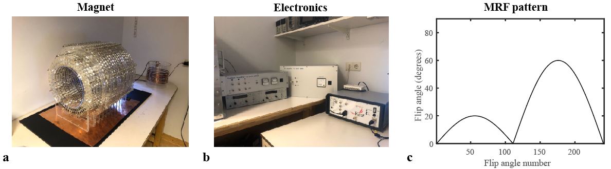
Magnet: The system used was a 50 mT Halbach magnet consisting of 23 rings filled with neodymium boron iron magnets [1], shown in Fig. 1a,b. A 15 cm diameter, 15 cm long solenoid coil was used for single channel RF transmission and reception.MRF definition: A pattern of 240 flip angles (0°-60°) adapted from Ref. [2], was used, preceded by an inversion pulse with a delay of 24 ms (Fig. 1c). The TR/RF-phase was fixed to 12ms/0°. Repetition delays of 1s and 4s were implemented between MRF trains for in vivo and phantom scans, respectively.
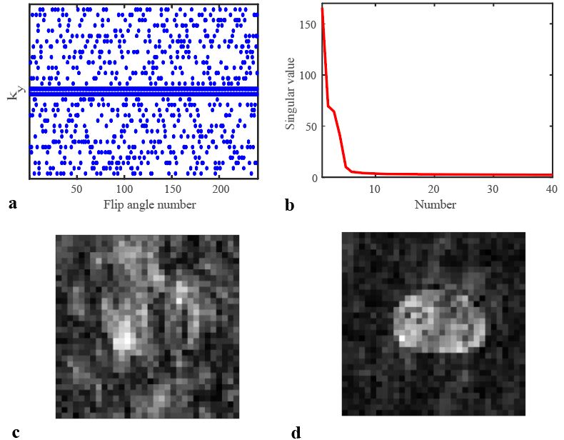
Data Acquisition: 3D MRF data was acquired in the lower arm of a healthy volunteer using a Cartesian sampling scheme in a spoiled SSFP sequence with an undersampling factor of 6. The 2x2 center region of k-space was always fully acquired in each MRF frame and serve as calibration data for matrix completion reconstruction [3] (Fig. 2a). Scan parameters: FOV 128x128x150 mm3, resolution 4x4x6 mm3, imaging bandwidth = 20.000 Hz and a scan time of 11 min and 18 min for in vivo and phantom, respectively. The readout direction was set along the bore and implemented with an oversampling factor of 2 to reduce foldover artifacts.
Dictionary, reconstruction and matching: The dictionary was calculated using the extended phase graph formalism [4]. 51832 signal evolutions were simulated with T1 and T2 values ranging from 20-1500 ms and 10-300 ms and a B1+ fraction ranging from 0.75-1.2, respectively. Acquired data were first reconstructed with matrix completion [3], using the first 5 singular vectors of the calibration data to form a projection matrix. Reconstructed images were then matched to the dictionary, while keeping the B1+ fraction fixed to the measured value.
Results
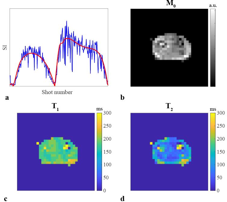
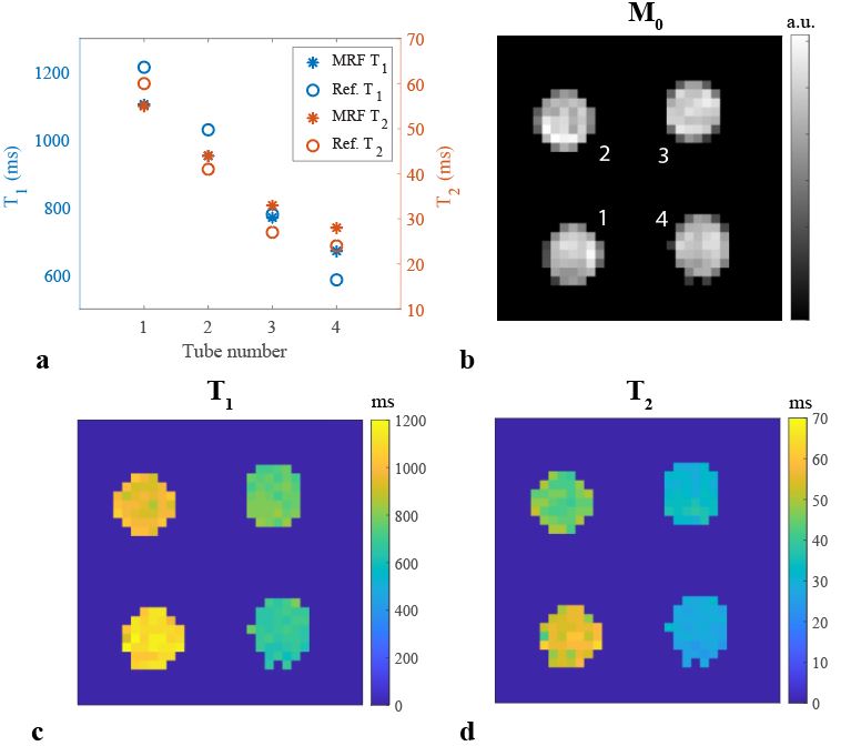
Figure 2b shows a steep decay in singular values calculated from the fully sampled calibration data in the MRF scan. Figure 2c shows the zero-filled reconstruction of one slice of a 3D volume at flip angle number 50 in the MRF train. Fig. 2d shows the same slice reconstructed with matrix completion, showing a substantial reduction in undersampling artifacts compared to the zero-filled reconstruction. The matched relaxation time maps (Fig. 3) report a T1/T2 of 180/50 ms in muscle. Relaxation times in a 4-tube phantom, shown in Fig. 4, are close to values obtained with reference techniques (non-selective IR and CPMG).Discussion
The first MRF measurements on our 50 mT system show a good match between measurement data and the simulated dictionary both in a phantom and in vivo. The measured relaxation times in muscle are in the same range as those measured with standard T1 and T2 mapping techniques [5]. Future work will focus on applying MRF in larger anatomies and investigate the effects of strong ΔB0 (~3000 Hz) and limited receiver bandwidth on the matched relaxation times. Sequence optimization for the relaxation times expected at low field strengths should extend the MRF sequence to larger FOVs and higher resolutions in a practical scan time (~10 min).Conclusion
3D Cartesian MRF with matrix completion reconstruction is possible using a 50 mT Halbach array. This can be used to obtain insight into relaxation times at low field and could therefore help to optimize MR sequences used on low field systems.Acknowledgements
This work is supported by the following grants: Horizon 2020 ERC FET-OPEN 737180 Histo MRI, Horizon 2020 ERC Advanced NOMA-MRI 670629, Simon Stevin Meester Award and NWO WOTRO Joint SDG Research Programme W 07.303.101.References
1. O’Reilly T et al. In vivo 3D brain and extremity MRI at 50 mT using a permanent magnet Halbach array. MRM. 2021;85(1):495-505.
2. Jiang Y et al. MR Fingerprinting Using Fast Imaging with Steady State Precession (FISP) with Spiral Readout. Magn Res Med. 2015;74:1621-1631.
3. Doneva M et al. Matrix completion-based reconstruction for undersampled magnetic resonance fingerprinting data. Magnetic Resonance Imaging. 2017; 41:41-52.
4. Scheffler K. A pictorial Description of Steady-States in Rapid Magnetic Resonance Imaging. Concepts in Magnetic Resonance. 1999;11(5):291-304.
5. O’Reilly T et al. High resolution in-vivo relaxation time mapping at 50 mT. Submitted to ISMRM 2021.
Figures