Introduction

Tissue susceptibility causes the polarising magnetic field (B0) in the head to be spatially varying and pose dependent¹, altering the signal acquired in MRI². Although having limited effect for small motion³ or clinical field strengths⁴, these B0 drifts hamper motion correction for increased motion levels at ultra-high field (UHF) and need to be included in the forward model⁵. Navigators and NMR probes have been used to measure pose-dependent fields but require additional hardware and/or scanning time and usually have limited temporal or spatial resolution^6,7. This work extends the DISORDER motion correction framework⁴, which leverages optimized Cartesian sampling, by including a physics-based model to account for pose-dependent B0 fields, resulting in a fully data-driven, retrospective motion correction.

Methods

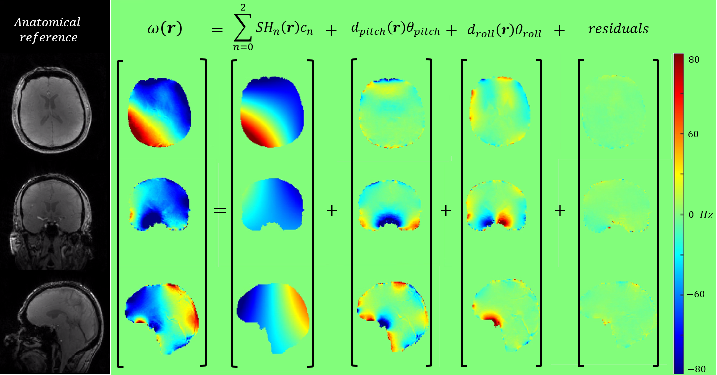
For volumetric encoding with Cartesian sampling, the DISORDER framework achieves motion correction by dividing k-space profiles (readouts) in temporal segments and allowing each segment to have a distinct motion state. This allows high (sub-second) temporal motion reconstruction as parallel imaging provides an over-determined problem to solve. However, adding a volumetric voxel-based estimation of the spatially varying B0 at every segment would make the reconstruction under-determined and a more compact B0 representation is needed. Building on prior studies^8,9, we observed that relative changes in B0 fields in the moving head frame due to motion at segment $$$s$$$ consist of a background field, represented well by lower-degree (2 here) solid harmonics (SH), and localised fields close to air tissue interfaces, which are proportional to the pitch and roll rotation angles $$$\theta_{pitch}$$$ and $$$\theta_{roll}$$$ (Fig. 1):

$$\omega_s(\textbf{r}) = d_{pitch}(\textbf{r})\theta_{s,pitch} + d_{roll}(\textbf{r})\theta_{s,roll} + \sum_{n=0}^2 SH_n(\textbf{r}) c_{n,s}\qquad(1)$$

where $$$\textbf{d}(\textbf{r})$$$ are the linear maps in $$$\boldsymbol{\theta}$$$, $$$SH_n$$$ the set of the solid harmonics of degree n with segment-dependent coefficients $$$c_{n,s}$$$. $$$c_{n,s}$$$ includes pose-dependent B0 effects (e.g. head-body orientation) as well as pose-independent B0 effects (breathing, scanner drift, etc)¹⁰. Both linear maps $$$\textbf{d}(\textbf{r})$$$ are smooth and sparse in space, reducing their parameter space even further. B0 fields are estimated based on data-consistency and incorporated in the DISORDER joint image ($$$\boldsymbol{\hat x}$$$) and rigid motion ($$$\boldsymbol{\hat z_s}$$$) reconstruction by replacing the Discrete Fourier operator $$$\boldsymbol{F}$$$ with a field-dependent Fourier operator $$$\boldsymbol{F_{\omega_{s}}}$$$¹¹. For spoiled sequences, the latter reduces to $$$\boldsymbol{FP_{\omega_s}}$$$ where $$$\boldsymbol{P_{\omega_s}}$$$ is a segment-dependent phase term. By commuting $$$\boldsymbol{P_{\omega_s}}$$$ and $$$\boldsymbol{ST_{z_s}}$$$, the phase term is applied in the native image space (head frame), which is consistent with the $$$\omega_s(\textbf{r})$$$ definition:

$$\boldsymbol{\hat x},\boldsymbol{\hat z_s},\boldsymbol{\hat \omega_s} = argmin_{\boldsymbol{ x},\boldsymbol{ z_s},\boldsymbol{\omega_s}} \sum_{s'}||\boldsymbol{A_{s'} FST_{z_{s'}}P_{\omega_{s'}}x-y_{s'}}||_{2}^{2}\qquad(2)$$

where $$$s'$$$ sums over all segments and $$$\boldsymbol{T_{z_s}}$$$, $$$\boldsymbol{S}$$$, $$$\boldsymbol{A_{s}}$$$, $$$\boldsymbol{y_{s}}$$$ respectively represent rigid motion, coil sensitivities, sampled profiles and measured data for segment $$$s$$$, as defined in DISORDER⁴. The DISORDER iterative solver is augmented with a Gradient Descent optimizer for $$$c_{n,s}$$$ at every segment and a Fast Iterative Thresholding Algorithm (FISTA)¹² for the regularised $$$d(\textbf{r})$$$ update:

$$\boldsymbol{d^{i+1}} = argmin_{\boldsymbol{d}} \sum_{s'}||\boldsymbol{A_{s'} F S T_{z_{s'}}P_{\omega_{s'}}x-y_{s'}}||_{2}^{2} + ||\boldsymbol{d}||_1 + ||\boldsymbol{D}\boldsymbol{d}||_2^2 \qquad(3)$$

where $$$\boldsymbol{D}$$$ is the finite-difference operator to enforce smoothness. The proposed reconstruction was tested in simulations and validated in-vivo for a spoiled gradient echo (SPGR) sequence on a 7T scanner (MAGNETOM Terra, Siemens Healthcare, Erlangen, Germany). A volunteer was asked to deliberately move position every 20 seconds. Sequence parameters: 1.5mm isotropic resolution, 0.66s DISORDER motion resolution, TR=10ms, TE=5ms, flip angle FA=7$$$^{\circ}$$$, FOV=220×240×200 (IS/AP/LR), readout along IS, scan duration TA=2min57s with no repeats and no acceleration.

Results

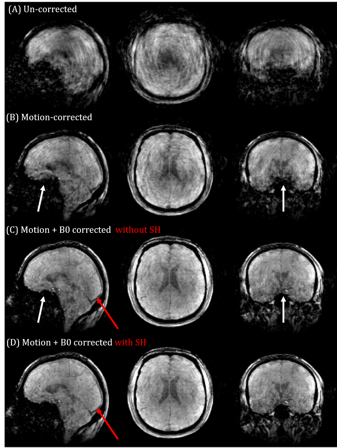
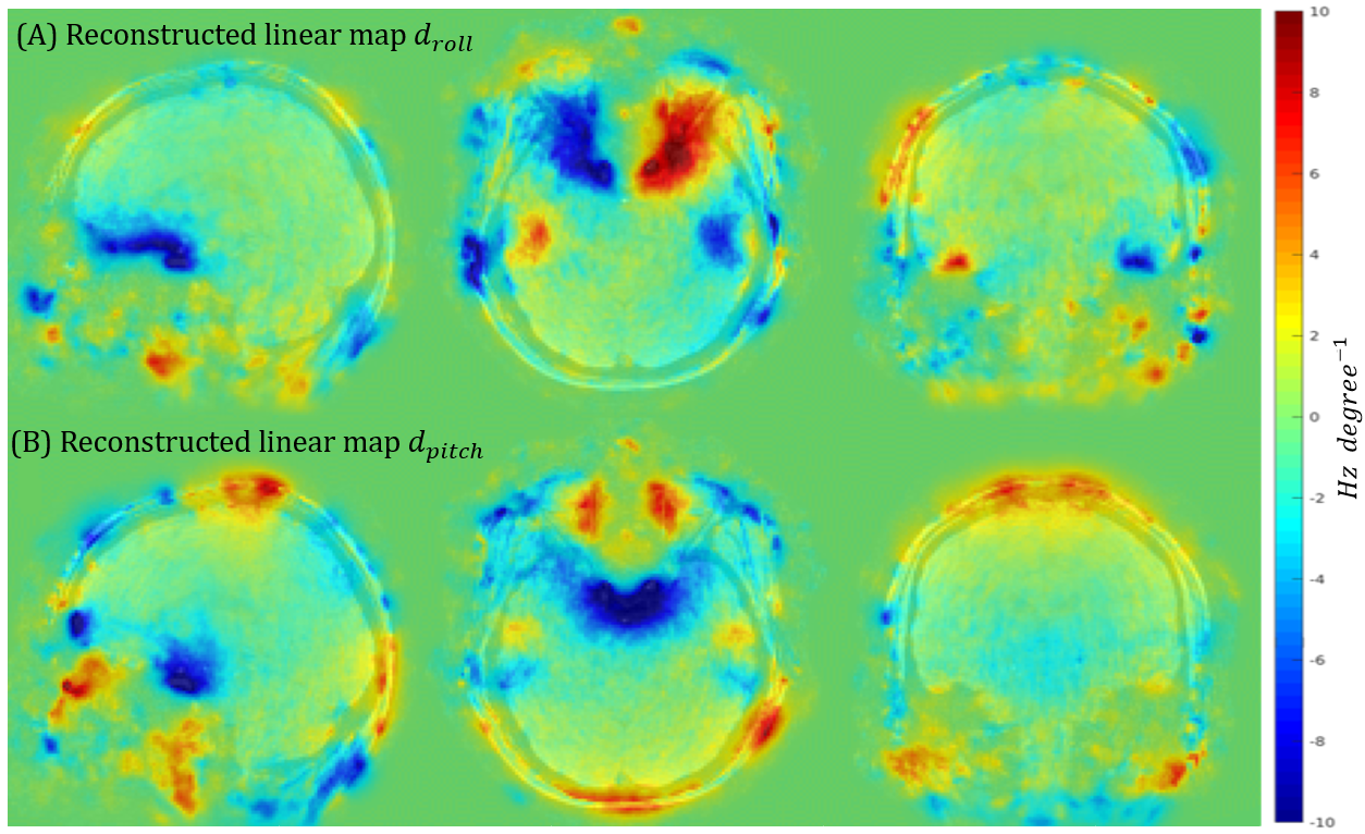
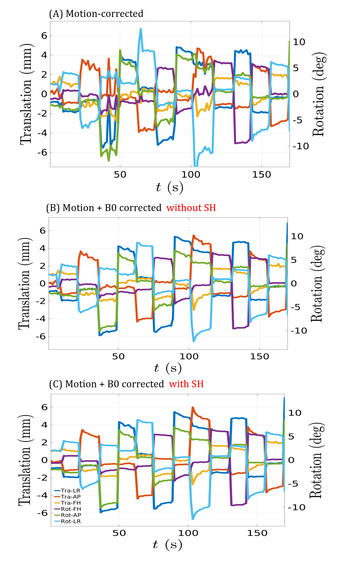
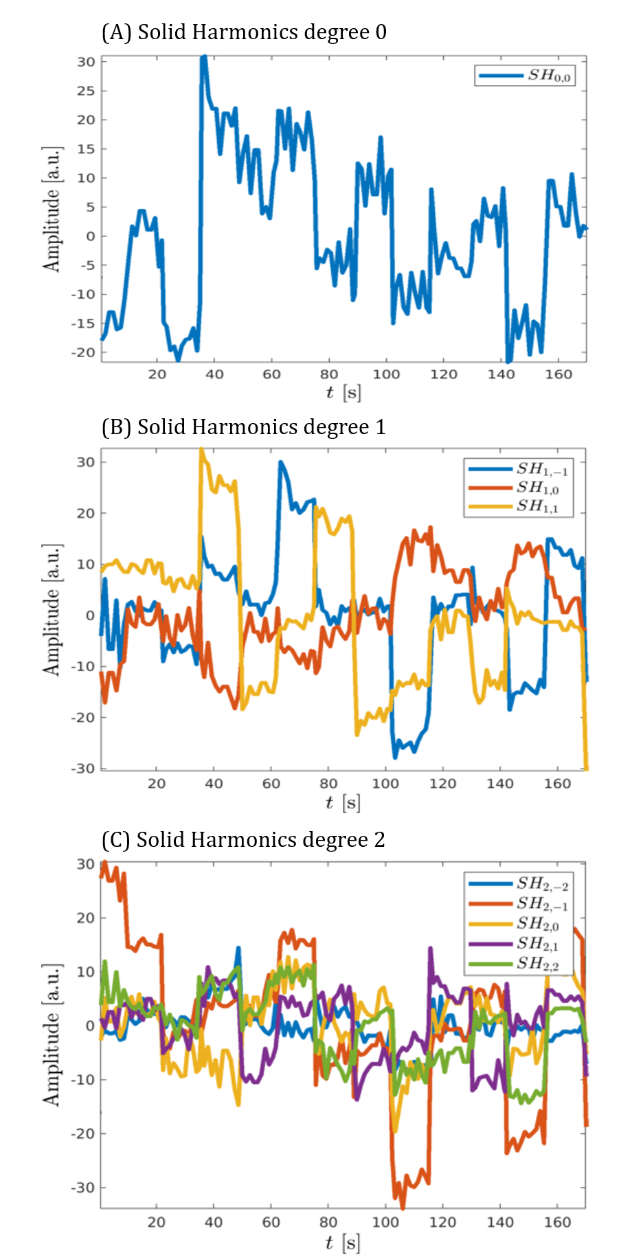
Fig. 2 shows magnitude images from the different reconstructions. A clear reduction in motion corruption is observed for the proposed motion and B0 corrected reconstructions. This results in an overall increase in contrast and a recovered signal in areas close to air-tissue interfaces. Only considering the SH does not greatly improve reconstruction (not shown), whereas the linear maps $$$d(\textbf{r})$$$ alone contribute most to the improved image reconstruction. Although motion corruption is reduced when accounting for B0 variation, the proposed reconstruction still contains residual artefacts and lower signal to noise ratio (SNR) compared to a motion-free scan. Linear maps $$$d_{pitch}(\textbf{r})$$$ and $$$d_{roll}(\textbf{r})$$$ are shown in Fig. 3 and agree with the literature^8,13,14 and our own observations from motion-free data both in terms of dynamic ranges (up to 10Hz/degree) and spatial distributions (near air-tissue interfaces). Estimated motion parameters for the different reconstructions are shown in Fig. 4. Including the B0 model in the reconstruction results in more stable and realistic motion traces. Finally, SH coefficient traces are shown in Fig. 5 and follow the motion pattern, with fluctuations superposed, which probably come from confounding factors (e.g. respiration), as previously suggested⁵. This confirms that $$$c_{n,s}$$$ includes pose-dependent and pose-independent effects.

Discussion

We have shown improved motion correction for UHF brain imaging by incorporating an explicit pose dependent B0 field term, using a compact physics-based model. Substantial reduction of motion artefacts was achieved in multiple test scans, however, as the conditioning of Equation (3) is determined by the variability of the motion parameters, simulations and in-vivo data show that the added benefit of the proposed reconstruction reduces in scans with little motion.

Conclusion

We have demonstrated the feasibility of fully data-driven retrospective rigid motion correction at UHF by including pose dependent B0 fields. Our method does not require any additional hardware or scanning time and once refined can be easily translated into other sequences.

Acknowledgements

The author would like to acknowledge funding from the EPSRC Centre for Doctoral Training in Smart Medical Imaging (EP/S022104/1).