0065
Compact Maps: A Low-Dimensional Approach for High-Dimensional Time-Resolved Coil Sensitivity Map Estimation
Shreya Ramachandran1, Frank Ong2, and Michael Lustig1
1Electrical Engineering and Computer Sciences, University of California, Berkeley, Berkeley, CA, United States, 2Electrical Engineering, Stanford University, Stanford, CA, United States
1Electrical Engineering and Computer Sciences, University of California, Berkeley, Berkeley, CA, United States, 2Electrical Engineering, Stanford University, Stanford, CA, United States
Synopsis
Dynamic MRI reconstruction techniques often use static coil sensitivity maps, but physical sensitivities can change substantially with respiratory and other subject motion. However, time-resolved sensitivity maps occupy a very large amount of memory, and hence, directly employing these maps is often impractical, especially on memory-limited GPUs. Here, we introduce a technique that solves for a compact representation of time-resolved sensitivity maps by leveraging a temporal basis for sensitivity kernels. Our proposed Compact Maps are significantly cheaper (by ~1000x) to store in memory than conventional time-resolved maps and result in lower calibration error and reconstruction error than do time-averaged maps.
Introduction
Parallel imaging1-4 is a widely used technique to accelerate scans, for which SENSE3-based reconstruction approaches require explicit knowledge of coil sensitivity maps. Dynamic MRI reconstructions often use a single set of sensitivity maps across time, which is estimated either from a calibration scan or a temporal average of the k-space data5. However, these static maps suffer from inaccuracies since sensitivities change with respiratory and other subject motion, as shown in Figure 1.Although previous works6,7 have calculated sensitivities frame-by-frame, this approach is challenging for iterative reconstructions with temporal constraints (such as total variation or low-rank regularizations). These reconstructions do not recover images frame-by-frame, but instead, continuously iterate through sets of frames to enforce temporal constraints. Hence, sensitivities cannot be computed on-the-fly and should be stored prior to the reconstruction. However, frame-wise sensitivities occupy a large amount of memory (see Figure 2), which often prohibits their use, especially on memory-limited GPUs. Therefore, we propose Compact Maps, a method that solves for a compact representation of time-resolved sensitivities using a low-dimensional approach.
Method
FormulationSince physical sensitivities are smooth in magnitude and phase, they have a compact representation in the spatial Fourier domain. To enforce this prior knowledge, we represent the maps as compact k-space convolution kernels. While maps change over time with motion, that change is smooth, and can be represented by a lower-dimensional temporal basis. Therefore, we define $$$(\hat{φ}_1,\hat{φ}_2,...\hat{φ}_N)$$$ as a temporal basis for the map kernels and $$$(\alpha_1,\alpha_2,...,\alpha_N)$$$ as corresponding basis coefficients (see Figure 3a, where $$$N$$$=3). To estimate these quantities, we perform a calibration using only central k-space data. The calibration jointly solves for the basis terms and a low-resolution image using an iterative SENSE8-like formulation, as shown below:$$(1)\hspace{0.5cm}\min_{m,\alpha,\hat{φ}}\sum_{i=1}^Tf(m,\hat{φ},\alpha)+R$$$$\textrm{where}\hspace{0.5cm}f(m,\hat{φ},\alpha)=\frac{1}{2}\|PF\{m_i\cdot(F^{-1}Z\sum_{j=1}^N\hat{φ}_j\alpha_{ij}^T)\}-y_i\|_2^2$$
Here, $$$m_i$$$ is the low-resolution image, $$$y_i$$$ is the low-resolution k-space data, $$$T$$$ is the number of time frames, $$$F$$$ is the 2D Fourier Transform, $$$Z$$$ is the zero-padding operation, $$$P$$$ is the projection onto the sampling pattern, and $$$R$$$ stands for the regularization terms, described further below.
Optimization
Although (1) is a non-convex problem, it is convex in each of $$$m$$$, $$$\hat{φ}$$$, and $$$\alpha$$$ when holding the other two quantities fixed. Therefore, we solve this problem with cyclic block coordinate descent, where each variable is updated individually by solving its corresponding convex subproblem. For large problems, we use stochastic optimization by randomly choosing a small batch of frames for each cycle (see Figure 3b).
The three subproblems for each variable update are as follows, where superscripts denote the cycle number:$$(2)\hspace{0.5cm}\alpha^{k+1}=\textrm{arg}\min_{\alpha}\sum_{i\in{batch}}f(m^k,\hat{φ}^k,\alpha)+\frac{\lambda_1}{2}\|D_t\alpha\|_2^2$$$$(3)\hspace{0.5cm}\hat{φ}^{k+1}=\textrm{arg}\min_{\hat{φ}}\sum_{i\in{batch}}f(m^k,\hat{φ},\alpha^{k+1})+\frac{\lambda_2}{2}\|W\hat{φ}\|_2^2+\beta^k\|\hat{φ}-\hat{φ}^k\|_2^2$$$$(4)\hspace{0.5cm}m^{k+1}=\textrm{arg}\min_m\sum_{i\in{batch}}f(m,\hat{φ}^{k+1},\alpha^{k+1})+\frac{\lambda_3}{2}\|m\|_2^2$$
In (2), $$$D_t$$$ represents a finite difference operator across time, which is used to impose temporal smoothness of the coefficients. Hence, the batches used for stochastic optimization must contain consecutive time frames. In (3), $$$W$$$ is a weighting matrix that enforces spatial smoothness by penalizing higher spatial frequencies in the basis components, inspired by the approach in ENLIVE9. The last term in (3) is a proximal point term10, which penalizes the difference between the updated variable value and its previous value to reduce noisy stochastic gradients. $$$\beta_k$$$ is increased for each epoch to gradually decrease the learning rate.
We use 3 iterations of conjugate gradient descent for each subproblem. Every time $$$\hat{φ}$$$ is updated, the Gram-Schmidt procedure is performed to orthonormalize the basis. We initialize $$$m$$$ with 1s, $$$\hat{φ}$$$ as 0s, and $$$\alpha$$$ as 1s. The optimization is warm-started by first using an 8x8 kernel size and $$$N$$$=1, then incrementally ramping these quantities up to the desired values with each warm start step. The described optimization was implemented in Python using the SigPy11 package.
Evaluation
With IRB approval, we acquired a 2D axial bSSFP dataset from a healthy volunteer on a GE 3T MR750W (3.5ms TR, 1.4x1.4mm spatial resolution, 0.5s temporal resolution). The dataset had 150 time frames, 18 channels, and 192x154 image matrix size. Retrospective undersampling of R=3 was performed by uniformly discarding phase-encode lines outside a calibration region of 20 lines. For the optimization, we used $$$N$$$=4 basis components, 24x24 kernel size, batch size of 5 frames, and 72x72 of central k-space data. The stochastic optimization was run for 20 epochs, after 5 epochs for each of three warm start steps. On a Nvidia Titan-Xp GPU, the calibration pipeline took ~500MB GPU memory and ~2min runtime.
Results
To evaluate the quality of Compact Maps, we compare them against time-averaged and frame-wise maps calculated using ESPIRiT4. In Figure 4, we use the calibration error metric12, which is the residual after projecting fully-sampled data onto the span of normalized sensitivities. Compact Maps achieve much lower calibration error than do time-averaged maps and perform similarly to frame-wise maps.For Figure 5, images are reconstructed using iterative SENSE with l2-regularization of λ=0.001. For time-averaged maps, residual aliasing artifacts are visible in the reconstructed images and in the difference with the reference, but are significantly reduced in those for Compact Maps. Compact Maps also result in a lower normalized root-mean squared error (NRMSE).
Conclusion
We have introduced a method that solves for a compact representation of time-resolved coil sensitivity maps to dramatically reduce their size in memory. Compact Maps can enable improvements in image quality for dynamic MRI reconstructions.Acknowledgements
We thank the following funding sources: NIH R01EB009690, NIH R01HL136965, NIH R01EB026136, NIH U01 EB025162, and GE Healthcare.References
- Sodickson, D. K. & Manning, W. J. Simultaneous acquisition of spatial harmonics (SMASH): fast imaging with radiofrequency coil arrays. Magn. Reson. Med. 38, 591–603 (1997).
- Griswold, M. A. et al. Generalized autocalibrating partially parallel acquisitions (GRAPPA). Magn. Reson. Med. 47, 1202–1210 (2002).
- Pruessmann, K. P., Weiger, M., Scheidegger, M. B. & Boesiger, P. SENSE: sensitivity encoding for fast MRI. Magn. Reson. Med. 42, 952–62 (1999).
- Uecker, Martin et al. ESPIRiT--an eigenvalue approach to autocalibrating parallel MRI: where SENSE meets GRAPPA. Magnetic resonance in medicine vol. 71,3: 990-1001 (2014). doi:10.1002/mrm.24751
- Feng, L., Grimm, R., Block, K.T., Chandarana, H., Kim, S., Xu, J., Axel, L., Sodickson, D.K. and Otazo, R. Golden‐angle radial sparse parallel MRI: Combination of compressed sensing, parallel imaging, and golden‐angle radial sampling for fast and flexible dynamic volumetric MRI. Magn. Reson. Med., 72 : 707-717 (2014). https://doi.org/10.1002/mrm.24980
- Kellman, P., Epstein, F.H. and McVeigh, E.R. Adaptive sensitivity encoding incorporating temporal filtering (TSENSE)†. Magn. Reson. Med., 45: 846-852 (2001). https://doi.org/10.1002/mrm.1113
- Uecker, Martin et al. “Real-time MRI at a resolution of 20 ms.” NMR in biomedicine vol. 23,8: 986-94 (2010). doi:10.1002/nbm.1585
- Pruessmann, K.P., Weiger, M., Börnert, P. and Boesiger, P. Advances in sensitivity encoding with arbitrary k‐space trajectories. Magn. Reson. Med., 46 : 638-651 (2001). https://doi.org/10.1002/mrm.1241
- Holme, H.C.M., Rosenzweig, S., Ong, F. et al. ENLIVE: An Efficient Nonlinear Method for Calibrationless and Robust Parallel Imaging. Sci Rep 9, 3034 (2019). https://doi.org/10.1038/s41598-019-39888-7
- Asi, Hilal, and John C. Duchi. "Stochastic (approximate) proximal point methods: Convergence, optimality, and adaptivity." SIAM Journal on Optimization 29.3: 2257-2290 (2019).
- Ong F, Lustig M. SigPy: A Python Package for High Performance Iterative Reconstruction. In: Proceedings of the ISMRM 27th Annual Meeting, Montreal, Quebec, Canada, May 2019 p. 4819.
- Uecker, Martin, and Michael Lustig. “Estimating absolute-phase maps using ESPIRiT and virtual conjugate coils.” Magnetic resonance in medicine vol. 77,3: 1201-1207 (2017). doi:10.1002/mrm.26191
Figures
Figure 1 (animated gif). Examples of how coil sensitivity maps change with respiratory and subject motion. When the subject slightly rotates their body, the maps for all channels similarly rotate. Since Channel 15 and 17 are near the chest wall, their maps change more visibly with respiratory motion than the map for Channel 9, which is near the subject’s posterior. The reference images are reconstructed from a fully-sampled 2D axial bSSFP dataset. All sensitivities shown here have been estimated with ESPIRiT4.
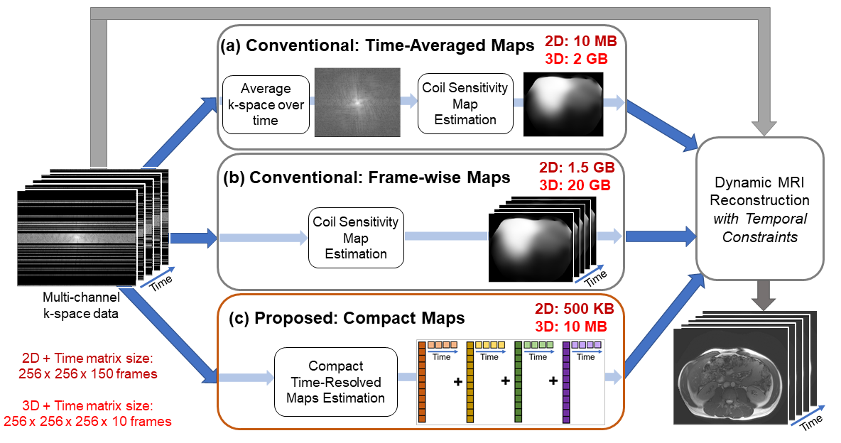
Figure 2. Overview of Compact Maps in a dynamic MRI reconstruction pipeline. Maps are generally pre-computed for reconstructions with temporal constraints, not computed on-the-fly. Conventionally, maps are estimated (a) from time-averaged k-space data or (b) individually for each time frame, then stored in the spatial domain. (c) Instead, Compact Maps are linear combinations of temporal basis components. Memory estimates are for $$$N$$$=4 basis components, 24x24 map kernel size, 8 channels, and the listed matrix size. We see ~1000x savings in memory with Compact Maps over (b).
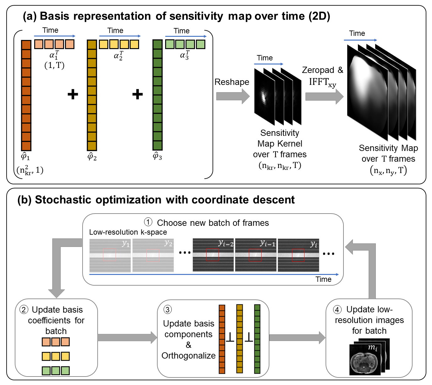
Figure 3. Illustration of method. (a) We solve for a basis representation of compact sensitivity kernels, which are the Fourier transform of sensitivity maps over time. Hence, nkr<<nx,ny. Here, we show $$$N$$$=3 basis components, denoted by different colors, and $$$T$$$=4 time frames. (b) In every cycle, a new batch of frames is chosen, and here, we show a batch size of 3 frames. Then the basis coefficients, basis components, and images are individually updated, and the basis is orthonormalized after its update. Update equations for steps 2,3,4 are listed as (2), (3), (4) in the text.
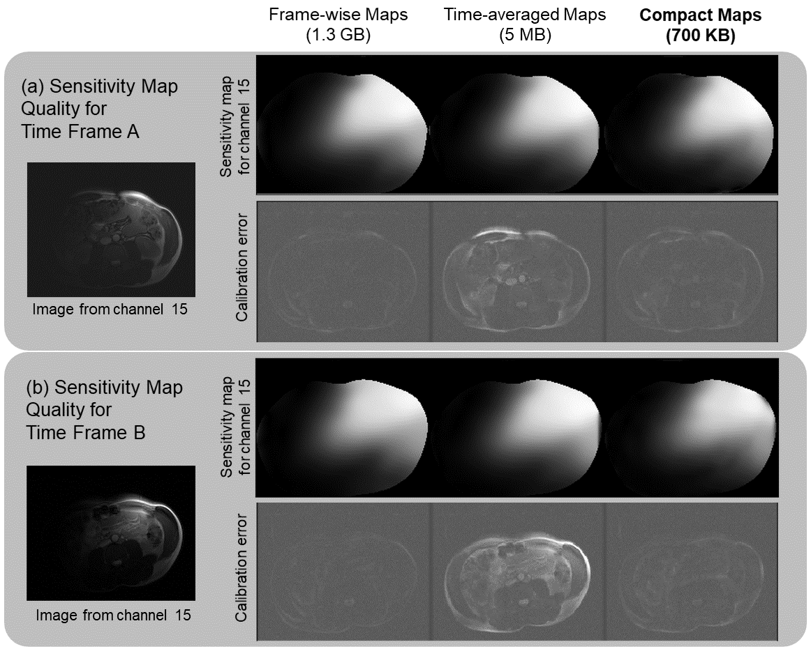
Figure 4. Comparison of sensitivity map quality of Compact Maps with ESPIRiT4 time-averaged and frame-wise maps. Calibration error is the residual after projecting fully-sampled coil images onto the span of the maps12 . Although the magnitudes of the maps appear to be similar, their different accuracies are captured in the calibration error metric. Two example time frames (A and B) show the significant reduction in calibration error for Compact Maps over time-averaged maps, but a similar performance to frame-wise maps even with a ~1500x reduction in memory.
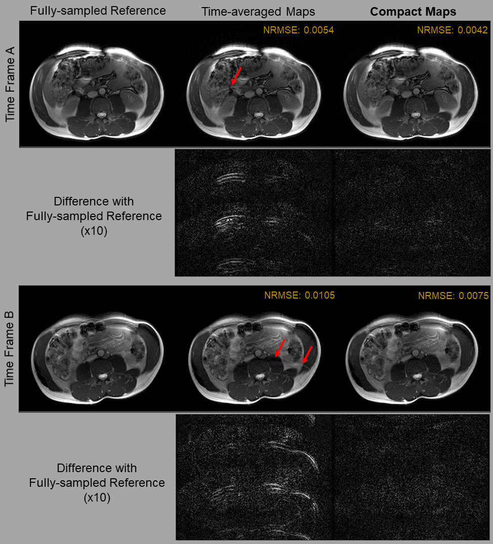
Figure 5. Comparison of image reconstruction quality using time-averaged maps and Compact Maps. Reconstruction has been performed for both time frames A and B using iterative SENSE with l2 regularization of λ=0.001. Difference images (x10) with the fully sampled reference are also shown. Residual aliasing artifacts are visible in images reconstructed with time-averaged maps (red arrows) and in the magnitude difference images, but are mitigated when using Compact Maps. Normalized root-mean square error (NRMSE) is also reduced in the images reconstructed using Compact Maps.