Target Audience

This talk is aimed at physicists and engineers who want to understand the different approaches used to simulate MR signals

Overview

The Bloch equations describe the evolution of nuclear magnetization in response to applied magnetic fields. MR pulse sequences typically consist of multiple pulses of both RF and gradient fields, and recovery periods; simulation of the magnetization dynamics throughout a sequence involves integration of the Bloch equations through time during such a sequence. These simulations are an essential tool for evaluating expected contrast (hence designing sequences) and quantitative approaches which seek to relate the observed magnetization response to underlying tissue properties. In order to fully characterise most pulse sequences it is not sufficient to consider the response of a single magnetization vector (or ‘isochromat’). Instead we must keep track of the behaviour of whole ensembles in order to recreate the ‘echoes’ that are key to the observed contrast from most sequences.
This talk will cover:

• Steady-state expressions
• Isochromat based simulation of general sequences
• Extended Phase Graph algorithm

Steady-state expressions

During a repeating pulse sequence lasting for much longer than the T1 and T2 times of the tissue, a steady-state is formed. Perhaps the best known example is the spoiled gradient echo sequence with repetition time TR and flip angle $$$\theta$$$, which will follow the Ernst equation:
$$ S=A \sin\theta \frac{(1-E_1)}{1-\cos\theta E_1} $$
where $$$E_1\equiv e^{\frac{-TR}{T_1}}$$$. This expression is straightforward to derive, under the approximation of perfect spoiling of transverse magnetization. In this case only the longitudinal magnetization forms a steady-state and the expression can be derived by considering only this single variable. As we will see later, this approximation breaks down when TR is not much larger than T2. It is possible to extend the same method of derivation to the case where the full vector magnetization must be considered, using a matrix-based framework. We will examine the general solution and apply it to balanced SSFP imaging.

Isochromat Ensembles

Balanced SSFP was used as an example in the previous section because it is a special case in which we may describe the magnetization within each voxel with a single magnetization vector. In general this is not the case, since the un-balanced gradient waveforms used in most pulse sequences lead to complicated distributions of magnetization at a sub-voxel level. Tracking of these distributions is essential if we are to accurately simulate the resulting signal. The simplest method for doing so is to consider not one magnetization vector, but a whole ensemble of them spaced out across a voxel; in the rotating frame, each one then experiences a different amount of rotation by angle $$$\psi$$$ around the z-axis, due to the applied gradients:
$$\psi=-\gamma\int_0^\tau \mathbf{G}(t).\mathbf{r} dt$$
Each of these locations is assumed to contain spins that all experience the same Larmor frequency, and is referred to as an ‘isochromat’ (the name derives from Greek and literally means ‘the same colour’). Isochromats are much smaller than voxels, and are by definition considered to be well modelled by a single magnetization that follows the Bloch equations. The observed MRI signal can be modelled by summing over the isochromat ensemble. Figure 1 shows some example ensembles evolving over the course of a gradient echo sequence, with and without RF spoiling.We will consider how many isochromats are needed to model magnetization behaviour, and how we could understand the signal dynamics by looking at these.

Extended Phase Graphs

This commonly used simulation framework can be conceptually difficult to understand, and so this abstract will go into a little more depth to accompany the talk itself.
Simulation of MR signal requires us to characterise the complex sub-voxel magnetization distribution. This can be ‘sampled’ by using isochromat ensembles, but another approach is to instead characterise the ensemble by its Fourier spectrum over ‘configuration states’. The magnetization distribution $$$M_{xy}(\mathbf{r})$$$ and $$$M_{z}(\mathbf{r})$$$ can be written in terms of configuration states
$$ F_+(\mathbf{k}) = \int_V M_{xy}e^{-i\mathbf{k.r}}d^3\mathbf{r}\\ Z(\mathbf{k}) = \int_V M_{z}e^{-i\mathbf{k.r}}d^3\mathbf{r} $$
Where `V' represents the voxel. The observed signal is the integrated transverse magnetization over the voxel, i.e. it is $$$F_+(0)$$$. Sequences that have a repeating gradient structure will produce rather compact magnetization distributions in this domain. This can be seen by the form of the rotation around the z axis by angle $$$\psi$$$ due to the applied gradient, which could be rewritten as:
$$ \psi=-\gamma\int_0^\tau \mathbf{G}(t).\mathbf{r} dt = \mathbf{\Delta k . r} $$

The effect of this gradient on the configuration states is to shift the transverse configuration states such that $$$F_+(\mathbf{k})\rightarrow F_+(\mathbf{k+\Delta k})$$$; this is mathematically equivalent to rotating the transverse magnetization around the z-axis, which is what happens in the space domain. If the same gradient area is applied after each excitation then the only possible values of $$$\mathbf{k}$$$ that can occur are integer multiples of $$$\mathbf{\Delta k}$$$. In that case the magnetization can instead be written as the sum over a discrete set of configuration states: $$ M_{xy}(\psi)=\sum^\infty_{n=-\infty} F_n e^{in\psi}$$

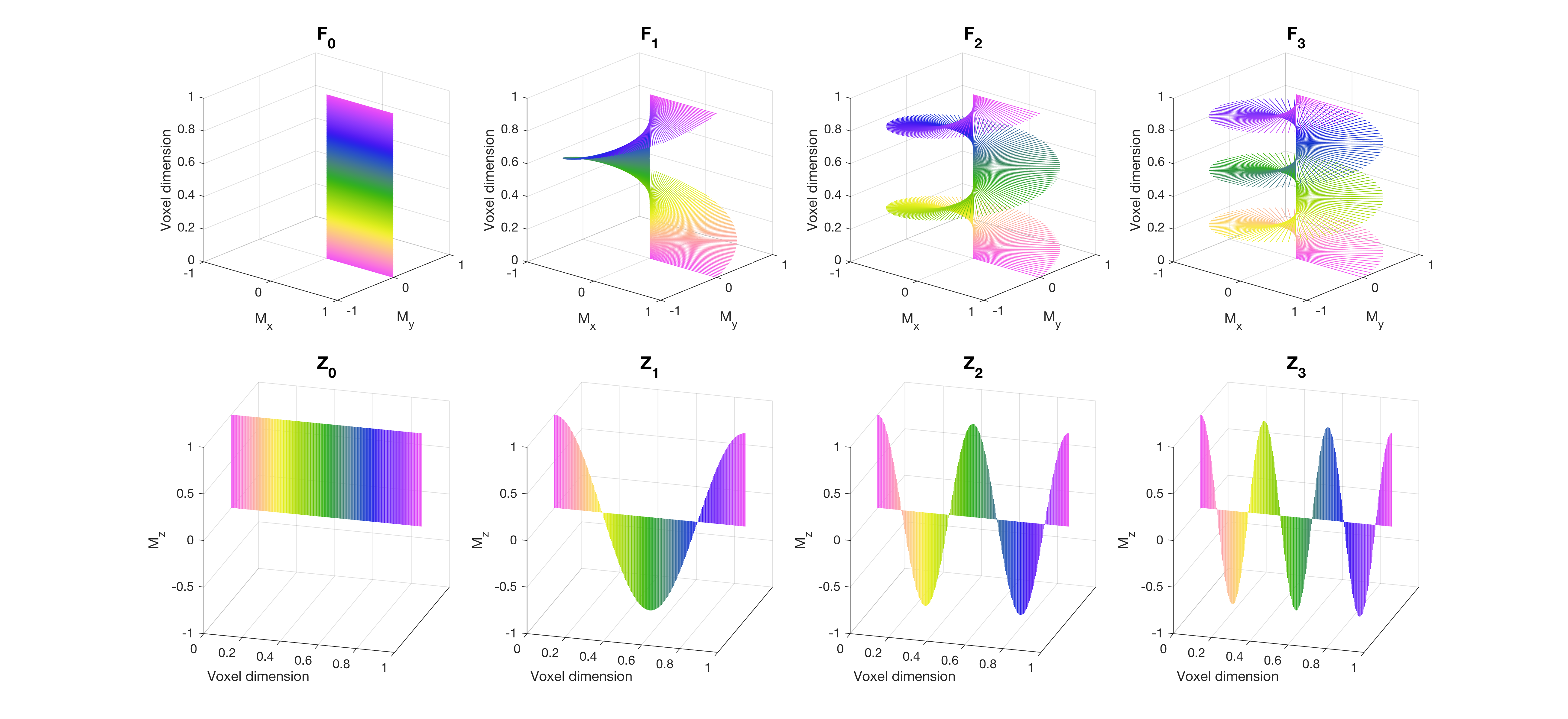
To fully understand the way that magnetization in the configuration states evolves through a sequence we also must consider the effect of RF pulses. In the isochromat domain an RF pulse causes the rotation of all magnetization vectors about some axis in the transverse plane, depending on the phase of the RF pulse. Crucially we consider the $$$B_1^+$$$ field to be uniform over the voxel, meaning that all isochromats in the ensemble are rotated by the same amount in the same direction. Hence an RF pulse cannot fundamentally alter the distribution of the magnetization, only rotate it. In the Fourier domain this means that an RF pulse will not `mix' configurations with different $$$\Delta k$$$; rather, RF pulses lead to a redistribution between longitudinal ($$$Z$$$) and transverse ($$$F$$$) configuration states with the same $$$\Delta k$$$. A fuller mathematical treatment will be given in the lecture; refer to [1] for an in-depth review.The configuration states can be visualised as representing magnetization with different spatial modulation across a voxel; $$$F_0$$$ and $$$Z_0$$$ represent spatially constant magnetization, for example. Assuming that $$$\Delta k$$$ imparts a phase of $$$2\pi$$$ across the voxel, all transverse configurations with $$$n\neq0$$$ average to zero and hence $$$F_0$$$ represents the observed signal. $$$F_1$$$ and $$$Z_1$$$ represent magnetization modulated by $$$2\pi$$$ over the voxel, $$$F_2$$$ and $$$Z_2$$$ have twice this modulation, and so on as illustrated by Figure 2.

The EPG algorithm can be used to make quantitative signal simulations by repeatedly applying some simple rules: 1. RF pulses mix together $$$F_n$$$ and $$$Z_n$$$ with the same $$$n$$$; 2. gradients shift $$$F_n\rightarrow F_{n+1}$$$; 3. Relaxation is applied separately to each configuration using the appropriate weighting (discussed in the talk). An example is given in Figure 3.

The EPG method is not inherently more computationally efficient than isochromat simulations for most operations. However an advantage is that the number of configurations that must be computed is well defined - we can see this by looking at the number of gradient periods. Perhaps more importantly, the EPG method allows us more \emph{insight} than isochromat simulations. We can see which `pathways' lead to echo formation, including more complex mechanisms such as stimulated echoes.

Summary

Signal simulations are an essential part of MRI sequence development, and increasingly also required for quantitative MRI methods. Magnetization dynamics can be modelled by integrating the Bloch equations. Closed form solutions can be found by seeking steady-state conditions in some cases. More generally the action of gradients disperses magnetization within a voxel, and this complex sub-voxel distribution must be characterised in order to model the MRI signal. A general method is to divide space into infinitesimal portions that experience the same field (`isochromats'), model their magnetization separately, then integrate the result. The EPG method is an elegant alternative that performs the Bloch simulation in a Fourier domain representation that can be more compact. Both methods could be extended to model other effects, such as diffusion [5] or MagnetizationTransfer and exchange [3].

Acknowledgements

No acknowledgement found.