MR Basics Recap: Signal Encoding & k-Space
1Stanford University Radiology, United States
Synopsis
In MRI, spatial localization is provided by the use of gradients, and augmented by use of RF coil arrays. Gradients impart a linear phase variation of the transverse magnetization of any magnitude and direction. The resulting acquired signal is the Fourier transform of the magnetization for the specific linear phase, known as the k-space location. With sufficient sampling of signal across k-space locations, an inverse Fourier transform can reconstruct the magnetization distribution, or image. The Fourier relationship between image and k-space signals offers tremendous intuition for imaging tradeoffs, including resolution, field-of-view, artifacts, the use of multiple coils, and signal excitation.
Learning Objectives
The main learning objectives of this presentation are:- Basic encoding: gradients, spatial harmonics and k-space
- Image vs. k-Space relationships: resolution vs. extent, FOV vs. density, PSF vs. apodization, coil roll-off vs. correlation, and others
- Temporal Effects: Off-resonance, phase inconsistencies, modulation
- Alternative k-space trajectories and properties
Basic Concepts
Once excited, transverse magnetization precesses at the Larmor frequency, though the baseline precession is often ignored and subtracted away for analysis, using a “rotating” reference frame. Gradients can induce a linear frequency variation in space. The gradient strength, duration and direction can be completely controlled, and it is useful to think in terms of $$$\gamma \overrightarrow{G}$$$ as a vector with units Hz/m. The frequency variation is $$$\Delta f = \gamma \overrightarrow{G} \cdot \overrightarrow{r}$$$, where $$$\overrightarrow{r}$$$ is the position vector. Furthermore, the magnetization can be expressed as a complex exponential $$$m(\overrightarrow{r}) e^{-2\pi i \Delta f t}$$$. A row of spins along a direction, in the presence of a gradient in that direction, is analogous to keys on a piano. Each resonates at a different tone. Just as a musician can recognize the tones from sound vibrations, the computer will resolve the spin distribution by Fourier transforming the overall signal.Signal Equations
The k-space signal is a Fourier transform of the magnetization density1. It is useful to develop this both intuitively and mathematically.1D Encoding: First, consider the case of only 2 spins in the system with one at the origin, and one elsewhere. We can first acquire a signal that is the sum of both spins. Next we turn on a gradient for exactly the time to induce 180° of phase in the spin away from the origin, then acquire a signal that is the difference of these spins. The spin density at the spin locations is reconstructed as half of the sum and half of the difference of the two signals. This is nothing more than a 2-point, 1-dimensional Fourier transform.
2D Encoding: This simple case is extended to 2 dimensions, with four spins A, B, C and D at the corners of a square where A is at the origin, and D is the opposite corner. Gradients in two different dimensions can be applied to induce 180° of phase to spins B and D or to C and D. By acquiring signals with no gradient, each of these two gradients separately, and with both gradients, we obtain four signals that are linearly independent combinations of the spins. This system is easily inverted to obtain the spin density, and this is a 2x2 Fourier transform.
General Equations: Mathematically, it is useful to consider phase masks applied to A, B, C and D, written as complex exponential phases. The signals are the forward Fourier transform, and the reconstruction is an inverse Fourier transform. This is easily extended to much larger matrix sizes (NxN) and to 3D encoding, but acquiring the appropriate number of signals. Figure 1 shows a 256x256 image and k-space signal. Each k-space location has a corresponding phase mask that varies in spatial frequency and direction. In general, the k-space signal is $$$s(\overrightarrow{k},t) = F\{m(\overrightarrow{r})\}|_\overrightarrow{k(t)}$$$ where $$$F\{\}$$$ denotes a Fourier transform and $$$\overrightarrow{k}(t) = \frac{\gamma}{2\pi} \int_0^t \overrightarrow{G}dt$$$. The signal received is the Fourier transform of the spin distribution, with the k-space location being given only by a time-integral of gradients. Note that the spin distribution is now assumed to be continuous. The k-space will be sampled at discrete locations, which must be taken into consideration later.
Cartesian Encoding
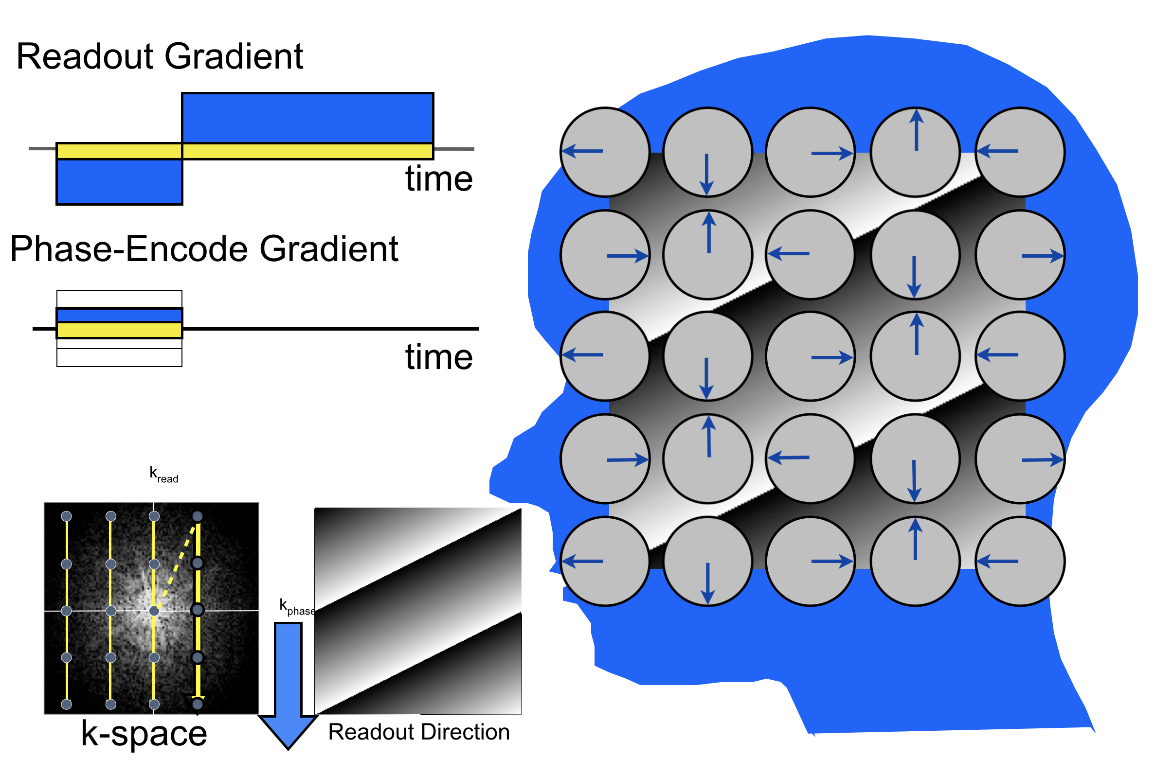
The most common type of k-space sampling, Cartesian sampling is shown in Fig. 22,3. A 2D image plane is divided into orthogonal frequency-encode (readout) and phase-encode directions. For each line, an initial (negative) readout gradient moves to the edge of k-space, while a phase-encode area moves to the desired line. During the readout, the phase-encode gradient is turned off, and the readout gradient provides sampling along a line. The phase mask changes along this line, and signal samples are collected, until the opposite extent of k-space is reached. The use of a sampling filter limits the range of positions that contribute signal to within a frequency-encode field-of-view ($$$FOV_x$$$). This sampling filter has a full bandwidth ($$$BW$$$) that is mapped to the readout direction FOV by the readout gradient ($$$G_x$$$) as $$$BW = \gamma G_x \times FOV $$$. On some systems the readout bandwidth is stated as bandwidth-per-pixel ($$$BW/N_x$$$), where $$$N_x$$$ is the number of pixels in the readout direction, while on others it is the “half-bandwidth” or $$$BW/2$$$.Image and k-Space Relationships
The Fourier transform relationship between image and k-space dictates many important relationships that must be considered in image acquisition:Resolution: Image resolution (pixel width) is the reciprocal of the k-space width. This applies generally to phase-encode and frequency-encode directions. It should be noted that k-space can be expressed in units of inverse pixels (between -0.5 and 0.5) or inverse length in any direction.
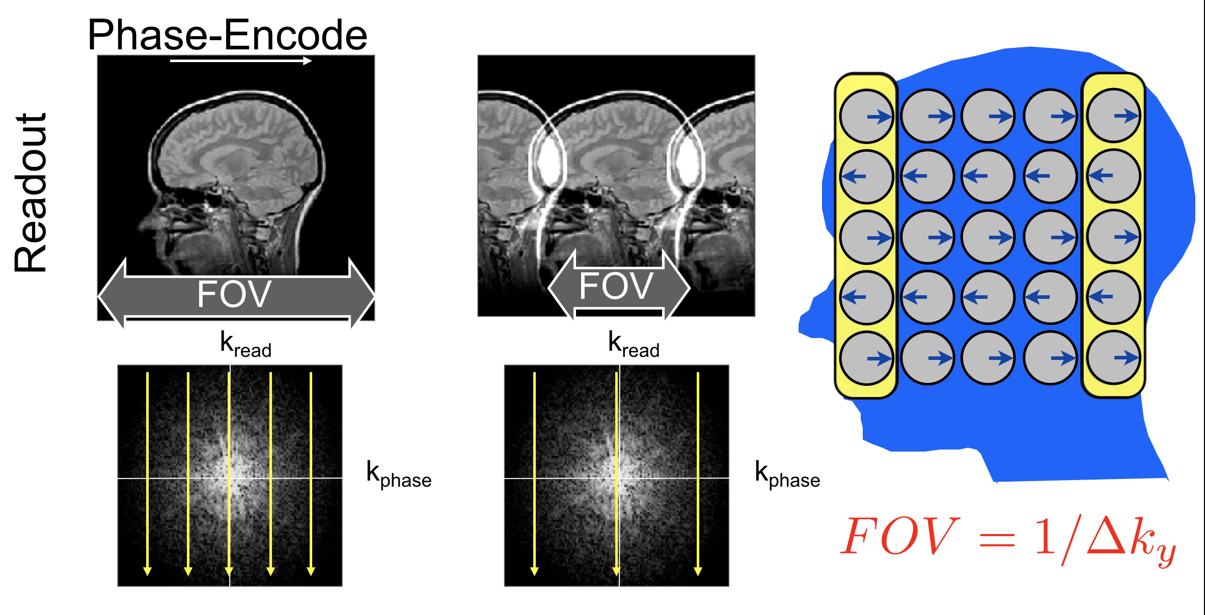
FOV: Image FOV is the reciprocal of the k-space sample spacing. In the frequency-encode direction, sampling at a rate equal to the full bandwidth (BW) matches this condition. In the phase-encode direction, the FOV is set by the k-space difference in phase-encode steps. This difference must be small enough for the FOV to encompass the object or aliasing will occur as shown in Fig. 3. Sufficient density is equivalent to sampling at the Nyquist rate.
k-Space Apodization and Ringing: Because the underlying spin distribution is actually continuous, the abrupt end of sampling at the extent in k-space leads to Gibbs ringing. Attenuating the signal at the edge of k-space (k-space apodization) can reduce this ringing at a cost of resolution.
Point-spread Function (PSF): Because the sample points can be considered as multiplying a continuous k-space, the inverse Fourier transform of the sample points gives the point-spread function. The PSF can represent all steps including sampling, apodization, and perhaps gridding interpolation, and is a compact illustration of resolution, FOV, ringing, and modulation effects.
Modulation Effects: The k-space signal magnitude and phase can be modulated by numerous effects including undersampling, T2 and T2* decay, off-resonance effects, object motion, and contrast enhancement. To the extent they are known, these can all be modeled into the PSF.
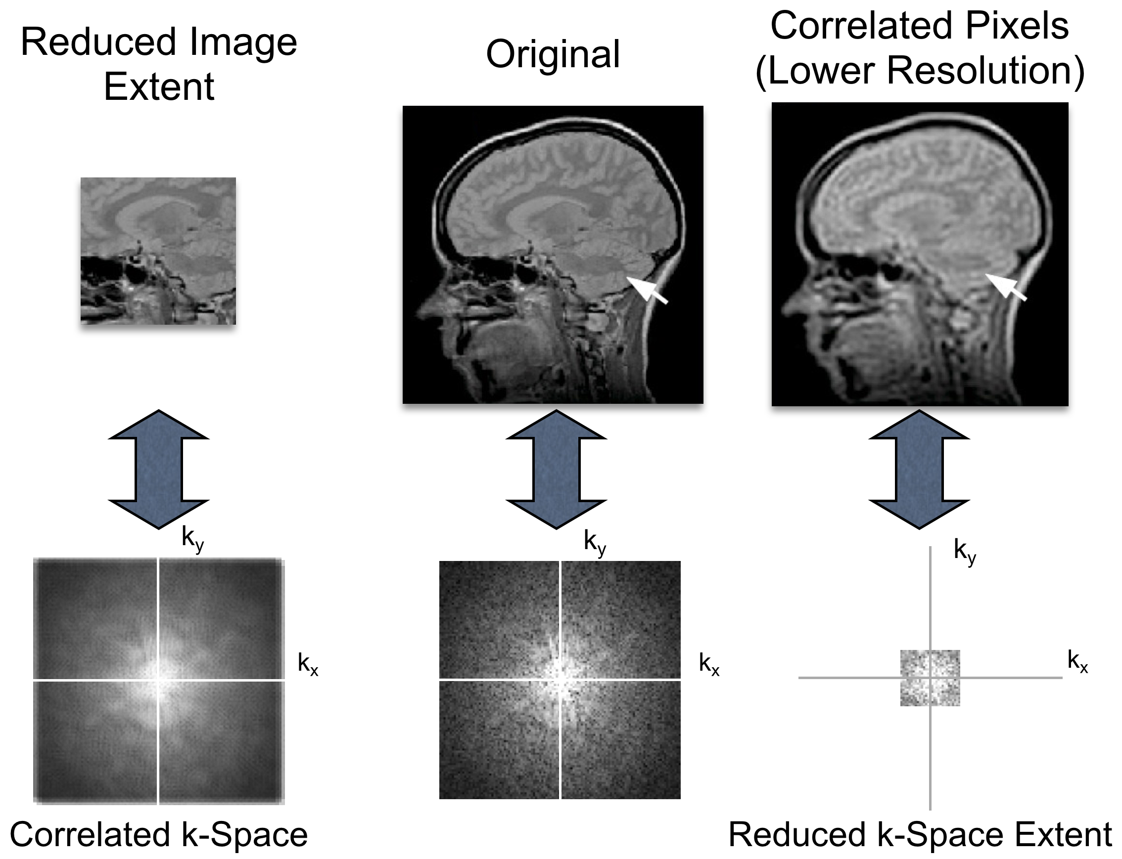
Figure 4 shows two important relationships. At right, reduced k-space extent leads to image blurring. If zeros are included beyond the extent, image interpolation results. At left, if the image extent can be limited (by finite excitation or coil sensitivity) the k-space is smoothed, enabling undersampling or providing correlations that can be exploited by parallel imaging methods such as GRAPPA.
Alternative k-space Trajectories
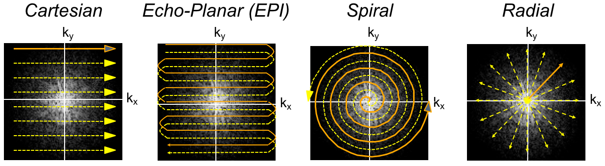
Efficiently sample k-space requires sampling many locations quickly. Fig. 5 shows some commonly used k-space trajectories. As the signal implies the trajectory is determined by the time integral of the gradient waveforms on each axis, which can vary over time. Compared to Cartesian sampling3, echo-planar imaging (EPI)4 and spiral5,6 can acquire much more k-space information from a single acquisition. Spiral and radial7 imaging can oversample the center of k-space, which can improve motion properties. Different trajectories have different characteristics with respect to undersampling, off-resonance, motion and system imperfections. Many trajectories collect samples that are not on a Cartesian grid, in which case interpolation to a grid (“gridding”) is used to enable a fast Fourier transform8. Alternatively, non-uniform fast Fourier transform (NuFFT) methods can be used. Radial sampling offers other approaches such as filtered back projection. EPI typically includes corrections for sampling in different directions and is arguably the most widely used alternative to Cartesian sampling. Extensive exploration of alternative k-space trajectories remains an active research area.Parallel Imaging
In parallel imaging, the sensitivities of multiple receive coils are used to improve image encoding, often enabling faster scanning or reduced modulation of k-space. Intuitively, in Fig. 3, if the signal can be obtained simultaneously from two coils placed at the front and back of the head, then knowledge of coil sensitivities can be used to unalias images. This is the basis of the SENSE approach9 – that FOV can be “built-up” from reduced-FOV images by coil arrays. Alternatively, the GRAPPA10 approach fills in missing lines in k-space by exploiting the correlations shown in Fig. 4. Numerous practical considerations and variations of parallel imaging methods enable routine use of parallel imaging in clinical scanning.Excitation k-Space
Similar to signal reception, a powerful excitation k-space formalism can be used11. Again, a time-integral of gradients determines the path through k-space, which instead ends at the k-space center. The excitation k-space “signal” is determined by the RF amplitude and phase as each location is traversed, and its Fourier transform gives the spatial excitation profile. Similar to parallel imaging, excitation k-space can be used with multiple transmit coils to formulate parallel transmit12, which can reduce excitation times or improve overall excitation profiles.Summary
MR images are primarily acquired by encoding position using gradients. Linear phase imparted by gradients enables a (conjugate phase) Fourier basis. The k-space signal is a map of the coefficients of each Fourier basis function, and sufficient sampling of k-space enables image reconstruction. Numerous Fourier relationships thus govern MR imaging, and many strategies for sampling k-space offer different tradeoffs.Acknowledgements
No acknowledgement found.References
1. Donald B. Twieg. The k-trajectory formulation of the NMR imaging process with applications in analysis and synthesis of imaging methods. Medical Physics, 10(5):610–621, September 1983.
2. Anil Kumar, Dieter Welti, and Richard R Ernst. NMR Fourier zeugmatography. Journal of Magnetic Resonance (1969), 18(1):69–83, April 1975.
3. W A Edelstein, J M S Hutchison, G Johnson, and T Redpath. Spin warp NMR imaging and applications to human whole-body imaging. Physics in Medicine and Biology, 25(4):751–756, July 1980.
4. P. Mansfield. Multiplanar image formation using NMR spin-echoes. J Phys Chem Solid State Phys, 10:L55, 1977.
5. C. B. Ahn, H. H. Kim, and Z. H. Cho. High-speed spiral-scan echo planar NMR imaging-I. IEEE Trans Med Imaging, MI-5:2, 1986.
6. C. H. Meyer, B. S. Hu, D. G. Nishimura, and A. Macovski. Fast spiral coronary artery imaging. Magn Reson Med, 28(2):202–213, 1992.
7. Paul G. Lauterbur and Ching-Ming Lai. Zeugmatography by reconstruction from projections. IEEE Transactions on Nuclear Science, 27(3):1227–1231, 1980.
8. J. I. Jackson, C. H. Meyer, D. G. Nishimura, and A. Macovski. Selection of a convolution function for Fourier inversion using gridding. IEEE Trans Med Imaging, 10(3):473–478, 1991.
9. K. P. Pruessmann, M. Weiger, M. B. Scheidegger, and P. Boesiger. SENSE: Sensitivity encoding for fast MRI. Magn Reson Med, 42(5):952–962, 1999.
10. M. A. Griswold, P. M. Jakob, R. M. Heidemann, M. Nittka, V. Jellus, J. Wang, B. Kiefer, and A. Haase. Generalized autocalibrating partially parallel acquisitions (GRAPPA). Magn Reson Med, 47(6):1202–1210, 2002.
11. J. Pauly, D. Nishimura, and A. Macovski. A k-space analysis of small-tip- angle excitation. J Magn Reson, 81(1):43–56, 1989.
12. Y. Zhu, C. J. Hardy, D. K. Sodickson, R. O. Giaquinto, C. L. Dumoulin, G. Kenwood, T. Niendorf, H. Lejay, C. A. McKenzie, M. A. Ohliger, and N. M. Rofsky. Highly parallel volumetric imaging with a 32-element RF coil array. Magn Reson Med, 52(4):869–877, 2004.
Figures
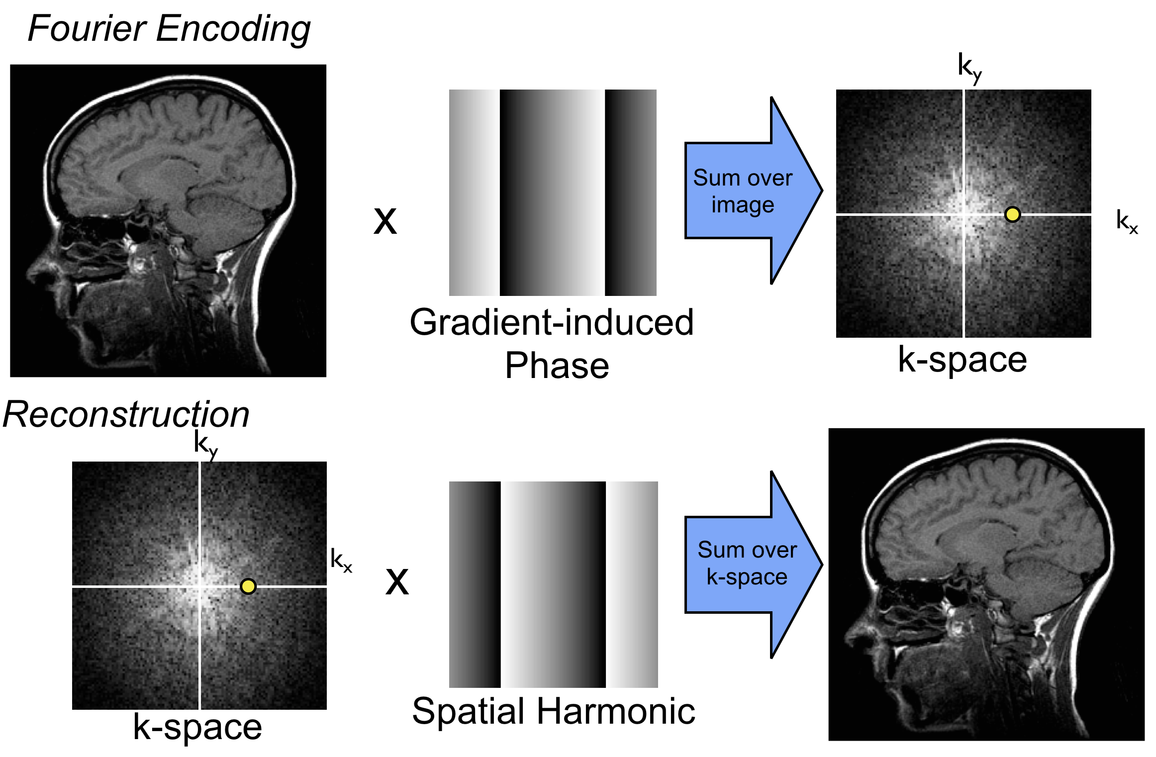
Figure 1. Fourier encoding and reconstruction: Gradients impart a linear phase pattern which is multiplied by the transverse magnetization. The sum of this product is the signal at a specific k-space location corresponding to the linear phase. The inverse Fourier transform used to reconstruct an image takes the k-space signal as a weight, that multiplies a linear-phase basis function. Summing this product over all k-space locations reconstructs the image.