4860
Quantitative Classification of Clinically Significant Prostate Cancer Using a Biexponential Model of Extended b-value Diffusion-Weighted MRI1Radiation Medicine & Applied Sciences, UC San Diego, La Jolla, CA, United States, 2Radiology, UC San Diego, La Jolla, CA, United States, 3Neurosciences, UC San Diego, La Jolla, CA, United States, 4Bioengineering, UC San Diego, La Jolla, CA, United States
Synopsis
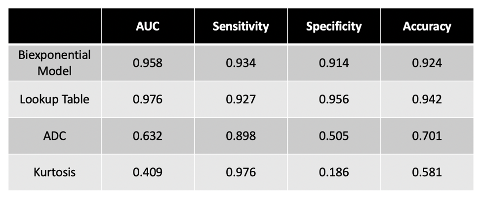
Prostate cancer is the second most frequent malignancy in men worldwide—novel strategies are needed to better identify patients with clinically significant disease. We developed a biexponential linear regression model using data from 36 men who underwent prostate MRI with 5 distinct b-values. We evaluated quantitative detection of clinically significant prostate cancer. The biexponential model and derivative lookup table outperformed simple ADC and kurtosis in quantitative classification of benign tissue and cancer (AUC 0.958 and 0.976 vs 0.632 and 0.409, respectively).
Introduction
Prostate cancer is the second most frequent malignancy in men worldwide and is a common cause of cancer deaths in men1. Strategies to improve outcomes for men with prostate cancer seek to optimize detection, staging, and clinical risk stratification.Clinical magnetic resonance imaging (MRI) currently includes diffusion-weighted imaging (DWI) and simple apparent diffusion coefficient (ADC) maps to determine a qualitative risk of clinically-significant cancer (PI-RADS v22). However, ADC is a measurement of overall diffusion rate of water within a voxel and can be influenced by multiple factors. It has shown correlation with presence of malignancy, but remains limited by motion sensitivity3, magnetic field inhomogeneity4, and high false-positive rates from inflammation, hemorrhage, or benign lesions that limit tumor conspicuity and localization3. Seventy-two percent of PI-RADS (v2) category 5 lesions yield a diagnosis of clinically significant cancer5.
Extended b-value diffusion imaging could improve microstructural characterization of cancerous and benign tissue6–8. Dependence of signal intensity on varying b-values can be modeled using linear combinations of exponential decay functions, with each component representing a diffusion element with a specific ADC, a framework called Restriction Spectrum Imaging (RSI). We developed a biexponential linear regression model and evaluated it for detection of clinically significant prostate cancer, as compared to ADC.
Methods
Study PopulationThis was a retrospective study of MRI data in men with suspected prostate cancer, collected between August and December 2016. Patients were selected if they had a benign prostate (defined as PI-RADS <3 or benign pathology) or if they had a biopsy-proven Gleason ≥7 prostate cancer visible on MRI (PI-RADS category 5).
MRI and Post-processing
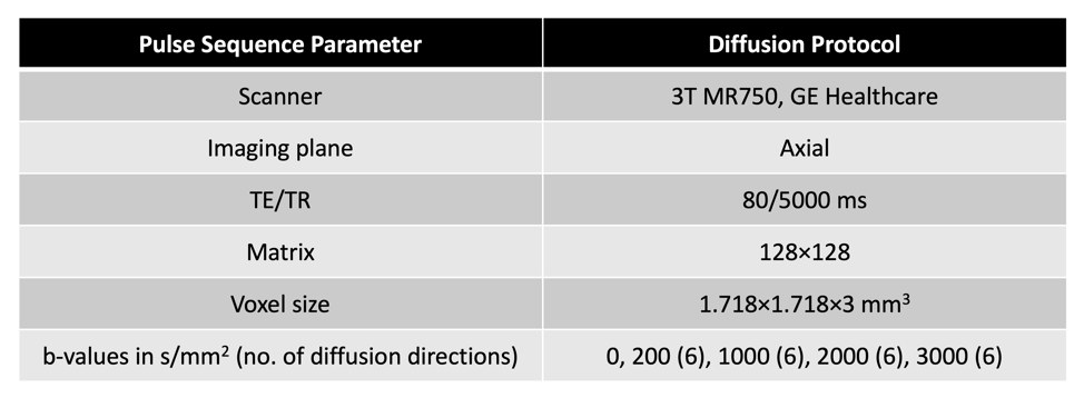
Scans were collected on a 3T clinical MRI scanner (Discovery MR750, GE Healthcare, Chicago, IL, USA), and the protocol included an axial T2W series (TE=100 ms, TR=6225 ms, in-plane voxel dimensions=0.4297x0.4297 mm, slice thickness=3 mm, field of view (FOV)=512x512) and a multi-shell diffusion series shown in Table 1. Diffusion data were corrected for distortions arising from B0 inhomogeneity9, and the T2W volume was resampled into diffusion space using an in-house algorithm developed in MATLAB (MathWorks, Natick, MA, USA).
Prostate Data Extraction
Benign voxels were defined as all diffusion data (full FOV) from patients without cancer. Cancer lesions were contoured by a radiation oncologist on diffusion images using MIM (MIM Software Inc, Cleveland, OH, USA). Contours were verified by a sub-specialist radiologist.
Biexponential Model of Prostate Diffusion
The relationship between corrected signal intensity and b-value was modeled as a linear combination of two exponential decays, where b represents diffusion weighting in s/mm2, f represents signal contribution of each component, and D represents the estimated ADC value for the population of voxels.
$$Signal\;Intensity= f_1 e^{-b*D_1} + f_2 e^{-b*D_2}$$
Differentiation Between Benign Tissue and Cancer
The model was evaluated using patient-level, leave-one-out cross-validation to generate a receiver operating characteristic (ROC) curve and corresponding AUC value. It was applied to the patients to generate a lookup table (LUT) indicating likelihood of cancer given f of each component for each voxel. ROC curves and AUC values for the model and LUT were then compared to those for simple ADC and kurtosis.
Results
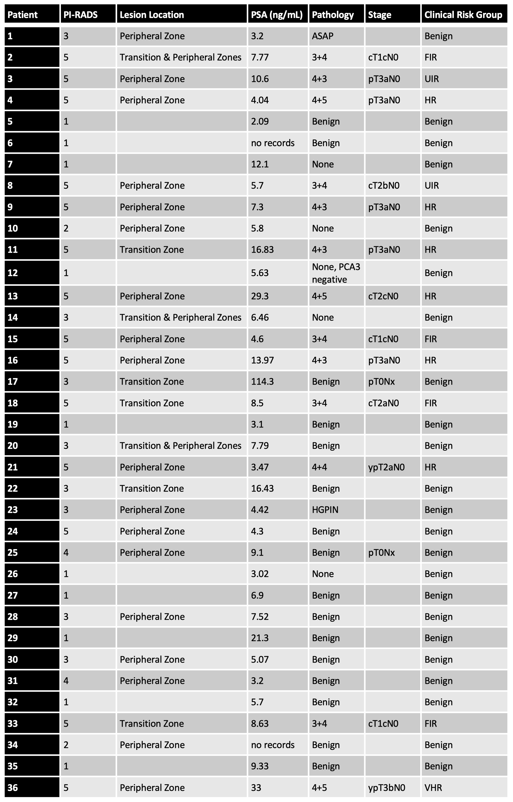
Sample SizeTwenty-three patients with benign prostates and 13 patients with clinically significant cancer were included in the analysis. Patient demographics are in Table 2. The number of voxels extracted from benign patients and cancer lesions was 7,378,101 and 3,361, respectively.
Differentiation Between Benign Tissue and Cancer
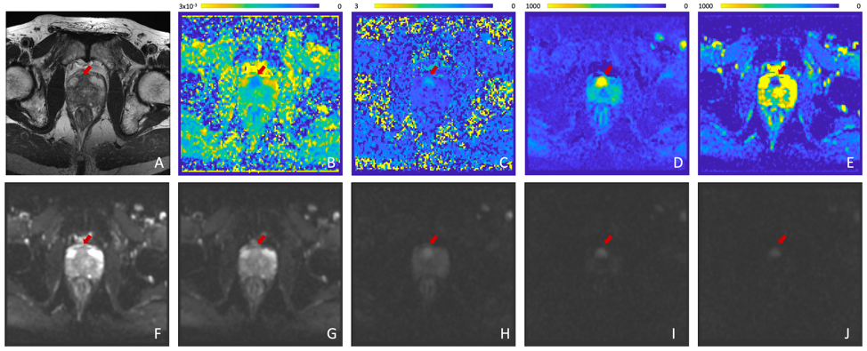
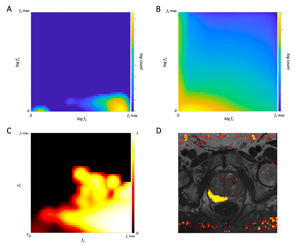
Optimal ADC values were estimated for the biexponential model in a preliminary study (not shown). Table 3 shows the AUC, sensitivity, specificity, and accuracy of the biexponential model, LUT, ADC, and kurtosis. Figure 4 is a representative axial slice of T2W, DWI, ADC map, kurtosis map, and f maps for each of the estimated components. Figure 5 illustrates f1 and f2 for the biexponential model, as well as the cancer-probability LUT and application to a representative image.
Discussion & Conclusion
The biexponential model and LUT performed best when compared to simple ADC and kurtosis. Kurtosis performed understandably poorly due to varying tissue types surrounding the prostate in the full FOV. Our biexponential model and LUT classified lesions correctly regardless of location in the prostate, unlike ADC10. A quantitative model has potential to improve reliability and objectivity by decreasing inter-reader variability and dependence on reader experience.A limitation is use of only PI-RADS 5 cancer lesions, which are already conspicuous to experienced radiologists. This may account for excellent performance seen using the biexponential model despite higher exponential models better accounting for the overall diffusion signal (not shown). In addition, despite our efforts to include only voxels with cancer in the contours, there appear to be portions of contoured cancer lesions that are not diffusion restricted, perhaps indicating necrosis within the tumor.
A biexponential model of diffusion and derivative LUT provide a high-confidence, noninvasive method of quantitatively distinguishing cancer from benign tissue. Future directions include optimization of multiexponential diffusion models for detection of radiographically occult prostate cancers, possibly including 3 or more exponential parameters, and evaluating performance in an independent dataset.
Acknowledgements
This study was funded by the U.S. Department of Defense (PC 160673), Prostate Cancer Foundation, UC San Diego Center for Precision Radiation Medicine, and NIH/NIBIB (K08 EB026503).
References
1. Bray F, Ferlay J, Soerjomataram I, Siegel RL, Torre LA, Jemal A. Global cancer statistics 2018: GLOBOCAN estimates of incidence and mortality worldwide for 36 cancers in 185 countries. CA Cancer J Clin. 2018;68(6):394-424. doi:10.3322/caac.21492
2. Turkbey B, Rosenkrantz AB, Haider MA, et al. Prostate Imaging Reporting and Data System Version 2.1: 2019 Update of Prostate Imaging Reporting and Data System Version 2. Eur Urol. 2019;76(3):340-351. doi:10.1016/j.eururo.2019.02.033
3. Kallehauge JF, Tanderup K, Haack S, et al. Apparent Diffusion Coefficient (ADC) as a quantitative parameter in diffusion weighted MR imaging in gynecologic cancer: Dependence on b-values used. Acta Oncol (Madr). 2010;49(7):1017-1022. doi:10.3109/0284186X.2010.500305
4. Koh D-M, Takahara T, Imai Y, Collins DJ. Practical aspects of assessing tumors using clinical diffusion-weighted imaging in the body. Magn Reson Med Sci. 2007;6(4):211-224.
5. Mehralivand S, Bednarova S, Shih JH, et al. Prospective Evaluation of PI-RADSTM Version 2 Using the International Society of Urological Pathology Prostate Cancer Grade Group System. J Urol. 2017;198(3):583-590. doi:10.1016/j.juro.2017.03.131
6. Shinmoto H, Oshio K, Tanimoto A, et al. Biexponential apparent diffusion coefficients in prostate cancer. Magn Reson Imaging. 2009;27(3):355-359. doi:10.1016/J.MRI.2008.07.008
7. White NS, Dale AM. Distinct effects of nuclear volume fraction and cell diameter on high b-value diffusion MRI contrast in tumors. Magn Reson Med. 2014;72(5):1435-1443. doi:10.1002/mrm.25039
8. Agarwal HK, Mertan F V., Sankineni S, et al. Optimal high b-value for diffusion weighted MRI in diagnosing high risk prostate cancers in the peripheral zone. J Magn Reson Imaging. 2017;45(1):125-131. doi:10.1002/jmri.25353
9. Holland D, Kuperman JM, Dale AM. Efficient correction of inhomogeneous static magnetic field-induced distortion in Echo Planar Imaging. Neuroimage. 2010;50(1):175-183. doi:10.1016/j.neuroimage.2009.11.044
10. Chatterjee A, Watson G, Myint E, Sved P, McEntee M, Bourne R. Changes in epithelium, stroma, and lumen space correlate more strongly with gleason pattern and are stronger predictors of prostate ADC changes than cellularity metrics1. Radiology. 2015;277(3):751-762. doi:10.1148/radiol.2015142414
11. Armstrong AJ, Victor AD, Davis BJ, et al. NCCN Guidelines Version 2.2019 Prostate Cancer.; 2019. https://www.nccn.org/professionals/physician_gls/pdf/prostate.pdf.
Figures