Introduction

Arterial-input-function(AIF) or vascular-input-function is the concentration of contrast agent in the blood plasma. AIF is a pre-requisite for the quantitative analysis of DCE-MRI data using various models for computing hemodynamic and tracer-kinetic parameters^1,2. Accurate estimation of AIF is challenging as it is a function of injection timing and dose, heart output rate, distribution of contrast agent, kidney function, partial volume effects and blood haematocrit(Hct). Several semi-automatic³ and automatic methods^2,4 have been reported for AIF estimation. Due to the advancement in MRI hardware and techniques, imaging protocols are being revised for higher spatial and temporal resolution. Depending upon imaging protocols and data quality, subject-specific AIF estimation approaches might result in erroneous curves. The objectives of the study were to improve the previously reported automatic AIF estimation method⁵, and evaluate its effect on quantitative DCE-MRI parameters as well as on differentiating high grade glioma(HGG) and low grade glioma(LGG)

Methods

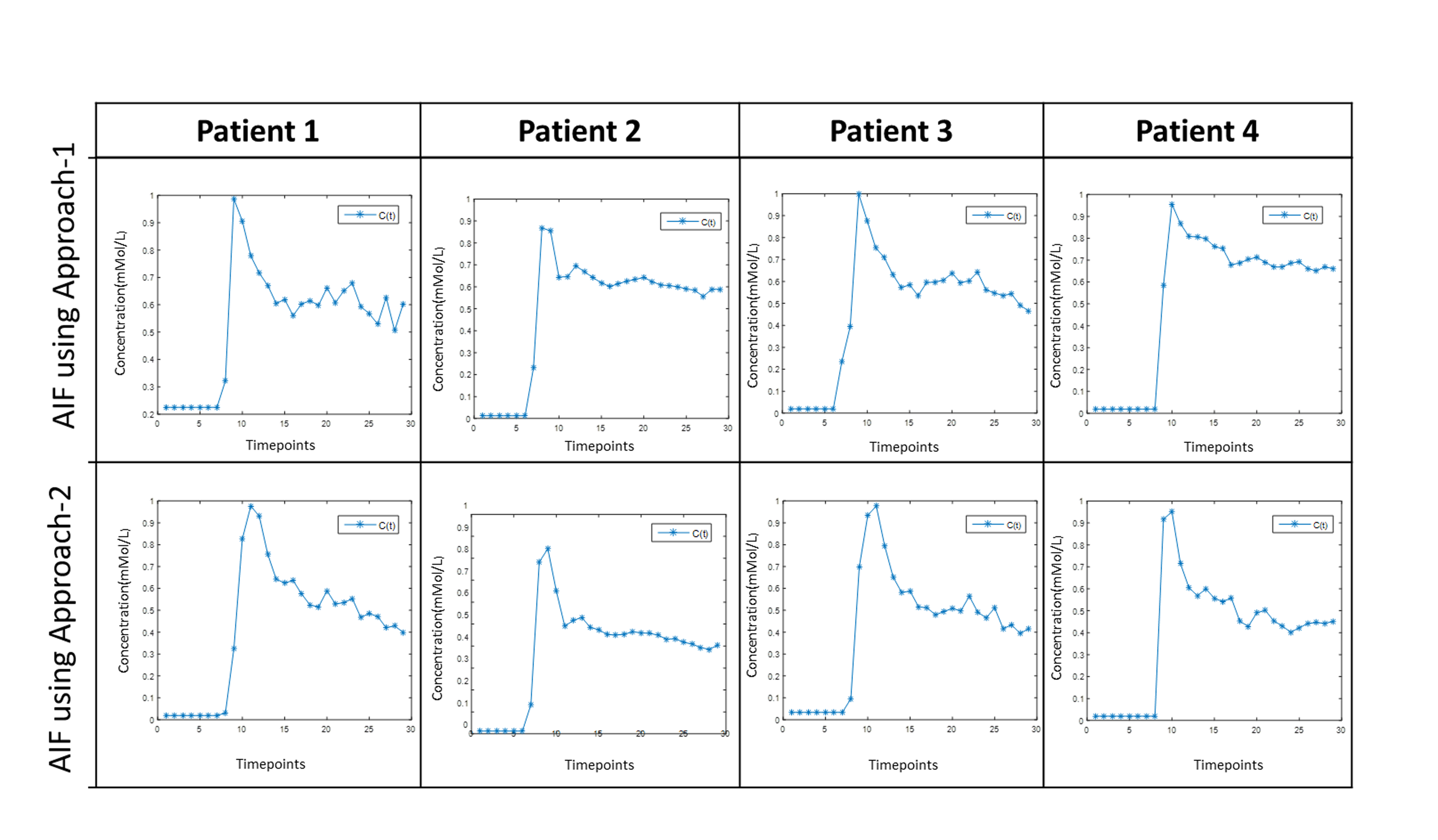
This IRB approved retrospective study included 25 patients (15 HGG and 10 LGG) with histologically confirmed Glioma(using WHO 2016 classification). MRI data included: conventional MRI, T1 map data and dynamic-contrast-enhance(DCE) or T1 perfusion MRI. MRI was performed at 3.0T scanner(Ingenia, Philips Healthcare, The Netherlands). Imaging Protocol: conventional MRI(T1-weighted, T2-weighted, FLAIR, post-contrast T1-weighted), and DCE-MRI(TR/TE=4.4/2.1ms, 10o FA, 240×240mm2 FOV, 12 slices with 6mm thickness, 32 dynamic with 3.9s temporality, contrast dose 0.1 mmol/kg body weight, 3.0ml/sec injection rate at 4th time point, contrast used Gd-BOPTA. A pre-contrast T1 map was generated and used for converting DCE-MRI signal-intensity-time curve to Concentration-time curve (C(t)) voxelwise². Piece-wise linear model was also fitted to extract parameters such as bolus-arrival-time (BAT), wash-out slope⁵, etc. Grading of glioma was done using perfusion parameters computed at combined contrast enhancing and non-enhancing area segmented using previously reported semi-automatic method⁶. Mean values greater than 90th percentile was used for grading. In this study, two approaches were used for automatic AIF estimation. Approach-1 implement the algorithm reported previously, Approach-2 introduces extra conditions in step-5 in Approach-1 as described below:
Step-1: Find (BAT), peak value, and time-to-peak(TTP) for each voxel’s C(t) curve.
Step-2: Threshold out all pixels with time difference[TTP-BAT] >15 seconds(~4 time points).
Step-3: Find the 98th percentile of the remaining voxels.
Step-4: Threshold out all pixels whose peak value falls below the 98th percentile. Step-5: Apply the following three conditions to remove the falsely selected voxels.
Step-5(a): The average C(t) values at the last few time points should be greater than 3 times the standard-deviation of C(t) at those time points.
Step-5(b): The average of C(t) at the last few time points should be greater than 3 times of standard-deviation of C(t) values before BAT.
Step-5(c): The peak value of C(t) should be greater than 2 times the average of C(t) at the last few time points.
Step-6: Match peak positions of the concentration curves at the remaining voxels.
Step-7: Take the average of concentration curves of all the finally selected voxels to get an averaged AIF.
The voxels which pass through these conditions were then averaged and normalized to generate final AIF. Values of AIF before BAT were replaced by the average of AIF values before its BAT. Final AIF is also normalized to mitigate partial volume effect. This algorithm was also tested for 99th percentile(Step-3). All images were descalped using SPM7. Generalized-Tracer-Kinetic-Model model was used to obtain kinetic parameters(Ktrans,Ve,Vp) and first pass analysis was used to obtain hemodynamic parameters(CBF, CBV) from C(t) curve. CBV(leakage corrected CBV)² and CBF used in this study were normalized using its mean value in the normal–appearing-white-matter tissue on the contralesional side (rCBV and rCBF)⁸. Quantitative parameters were estimated using AIF obtained using both methods were undergone ROC analysis for grading

Results and Discussion

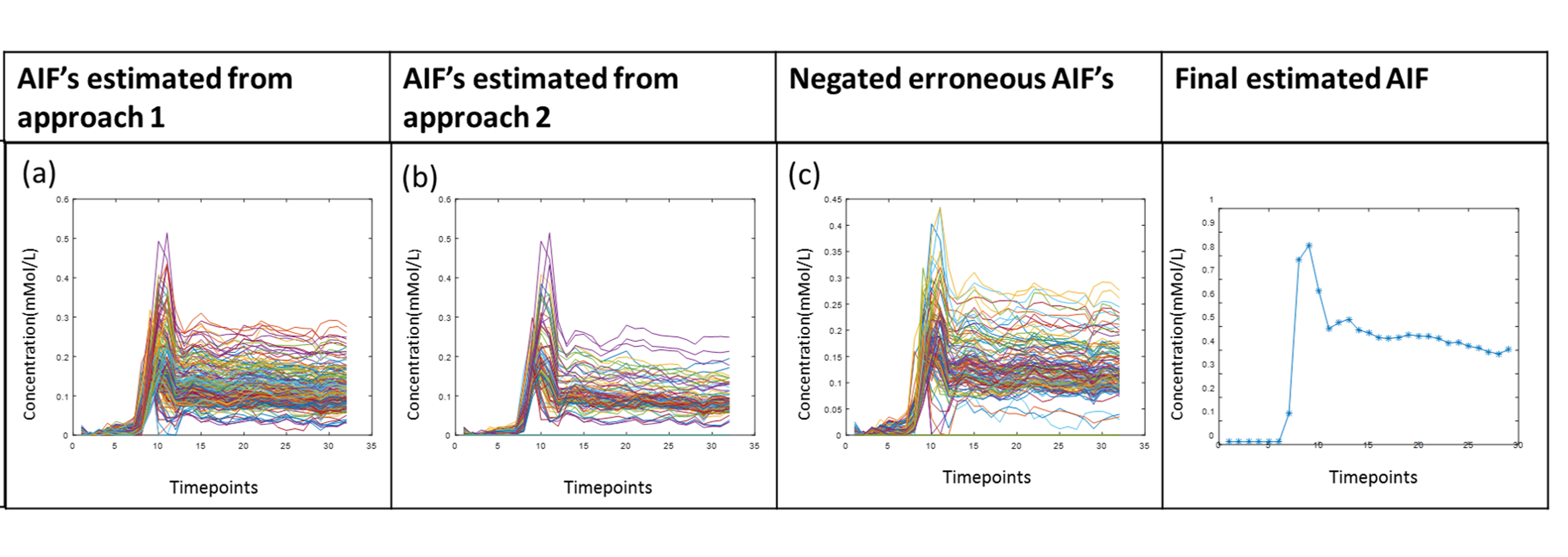
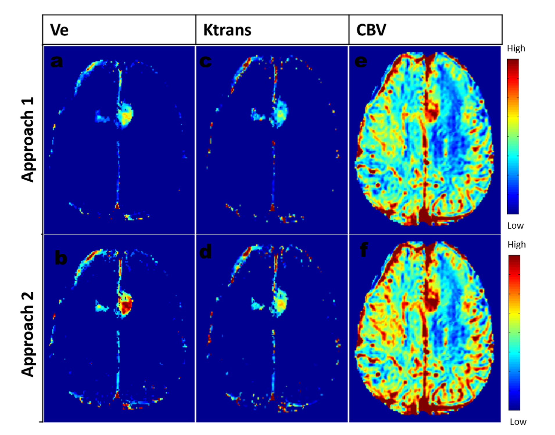
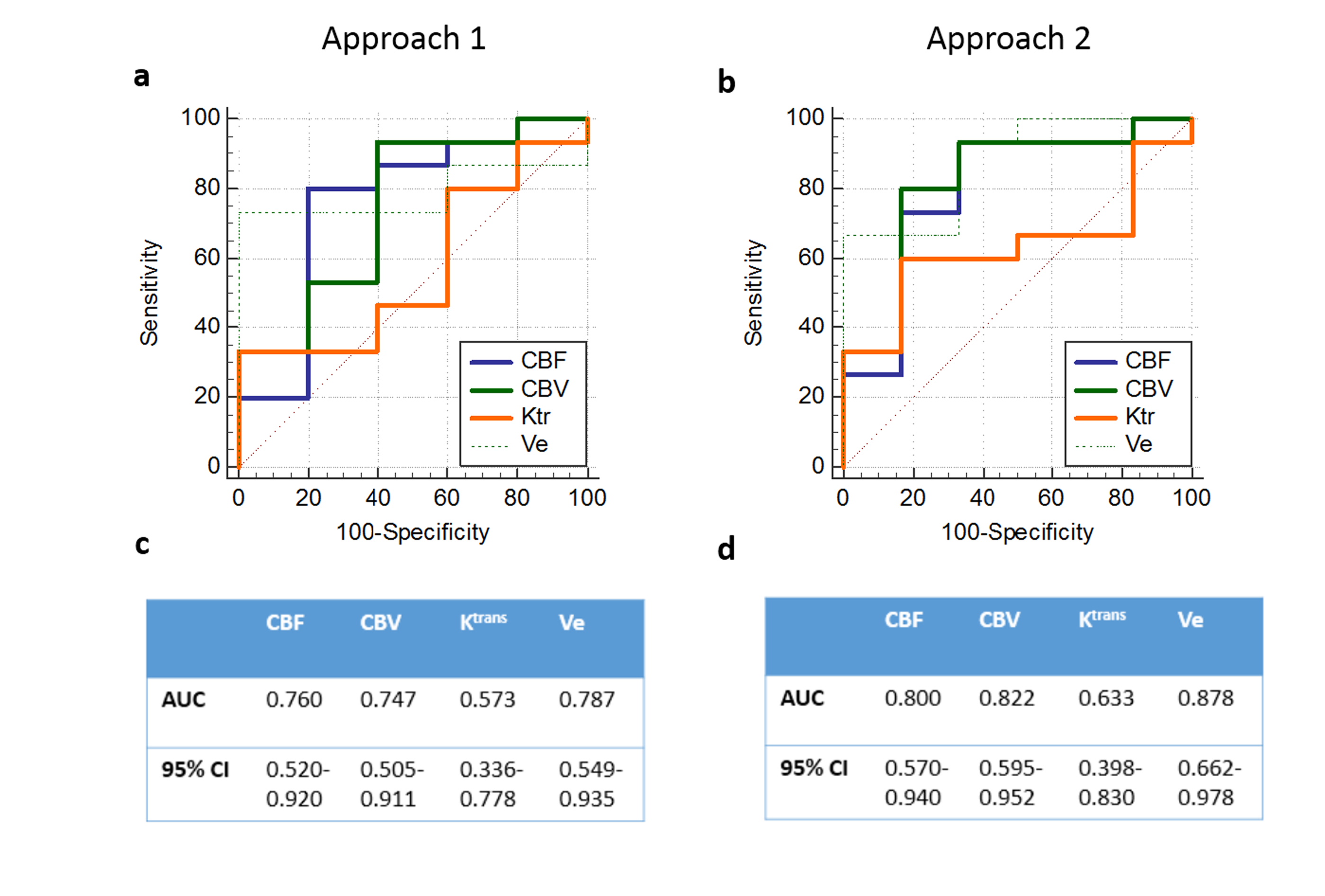
A large number of erroneous voxels selected using Approach-1 before averaging showed distorted shapes in AIF, which were successfully removed by the proposed optimizations introduced in Approach-2(Figure-1 and 2). The AIFs estimated using approach-2 were relatively smoother and closer to the shape of theoretical AIF than those estimated using Approach-1(Figure-1). Moreover, the shapes of averaged AIF using Approach-2 also showed less inter-subject variability in-terms of first pass and wash-out slope compared to those obtained using Approach-1. Ktrans, Ve and CBV maps obtained using both approaches are shown in figure-2. Estimation of CBV and Ve showed significant change(p=0.014 and p<0.001) while using proposed optimizations, which was reflected in ROC analysis(figure-4). As shown in figure-4 (c) and (d), area under ROC curves for differentiating LGG and HGG were improved for all parameters while using proposed method. Final AIF estimated using 98th and 99th percentile were almost overlapping.
The constraints applied in our method helped to individually identify only those voxels to be chosen that are physiologically correct and follow the traits of C(t) in the blood vessel. Proposed Approach-2 was tested on data from 25 patients with brain tumor and showed significant improvement. In future, it shall be tested on data sets acquired using different protocols at different scanners.

Conclusion

The proposed approach for AIF estimation successfully removed erroneously selected concentration-time curves and hence improved the accuracy and robustness of the final AIF. Statistically significant improvement in perfusion parameters were observed, which resulted in improvement of glioma grading.

Acknowledgements

This work was supported by Science and Engineering Research Board (IN) (YSS/2014/000092). The Authors acknowledge technical support of Philips IndiaLimited and Fortis Memorial Research Institute Gurugram in MRI data acquisition. The authors thank Dr. Mamta Gupta for data handling.