Introduction

Radiological assessment for breast cancer screening and diagnosis requires a series of dynamic contrast-enhanced images (DCE-MRI) to visualize areas of signal enhancement with sufficiently high spatial resolution to describe tumor boundary shape and structure. Acquiring these images with high enough signal to noise ratio (SNR) comes at the cost of requiring longer volumetric acquisition times, between 60-90 seconds per volume. More quantitative assessment of signal enhancement has been shown to improve (for example) specificity in distinguishing benign from malignant lesions¹. Estimating pharmacokinetic (PK) parameters with less than 10% error requires acquisition times to be at or below 16 seconds per volume of coverage². The signal enhancement ratio (SER) is a semi-quantitative approach for characterizing uptake that improves specificity³ and is correlated to PK parameters under certain acquisition conditions⁴. Importantly, the SER requires only three acquisition time points, S₀, S₁, and S₂, where S₀ is pre-contrast, S₁ is nearly the time of peak flow, and S₂ is chosen far enough to discriminate between flow that is persistently increasing, flattens in a plateau, or drops with washout. The SER is then defined as the ratio of (S₁-S₀) to (S₂-S₀). SER post-contrast time points vary, with S₁ often falling around 1.5 minutes post-injection of the contrast agent, and S₂ at the last-acquired time point, often 6-7 minutes later. It has been shown that decreasing S₂ from 7.5 to 4.5 minutes reduces the imaging time needed for a SER measurement without diminishing the ability to discriminate between benign and malignant breast lesions⁵. In this work, we seek to identify a set of three time points that allow for direct estimation of PK parameters by presenting a new method of searching mathematical mappings between PK parameters and uptake level at various possible sampling times.

Methods

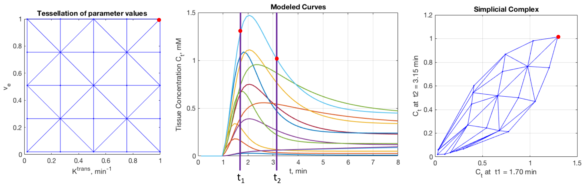
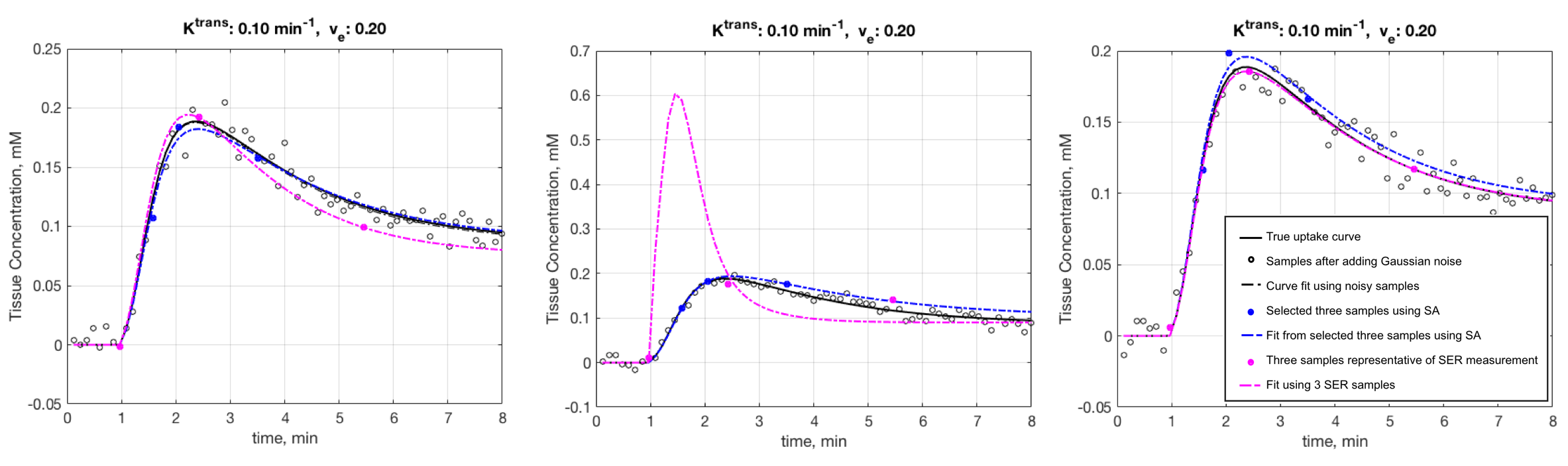
An analysis of simplicial complexes (ASC) was performed to select three time points at which to sample contrast agent concentration curves to maximize curve separation. The method can be used to select any number of time points, but is most easily visualized for 2-point selection as illustrated in Figure 1. For the standard Kety-Tofts model, parameter permutations of K^trans and v_e values are used to compute the set of associated tissue contrast-agent concentration curves using an available population arterial input function (AIF). Next, the set of all possible combinations of sample times is computed. For each sample time combination, a simplicial complex is generated whose vertices map to uptake curve values at the sample times (see Figure, 1 right panel.) The simplicial complexes are searched to select the one with maximum area, which indicates the best ability to discriminate between the curves. For the case of selecting three time points, simplicial complexes are curved surfaces in 3-dimensional space.
ASC was used to select three time points at 36, 65, and 153 seconds from injection using 21×21 (K^trans, v_e) permutations with values between 0 and 1. A second set of 961 (31×31) permutations of (K^trans, v_e) parameter values were used to generate simulated uptake curves by adding 10% Gaussian noise to computed curves. The addition of random noise was repeated 500 times to generate a test set of 480,500 noisy sample curves. The noisy sample curves were each sampled at the ASC time points of 36, 65, and 153 s and at another set of three time points that define the SER samples: 0, 90, and 270 s. For both sets of three-point samples, nonlinear least-squares fits to the standard Kety-Tofts model were used to generate fitted uptake curves and (K^trans, v_e) estimates. Figure 2 shows three examples of repeated generation of noisy curve samples for the entire time course, ASC and SER selected three-point samples, and the result of applying fits to both 3-sample sets.

Results

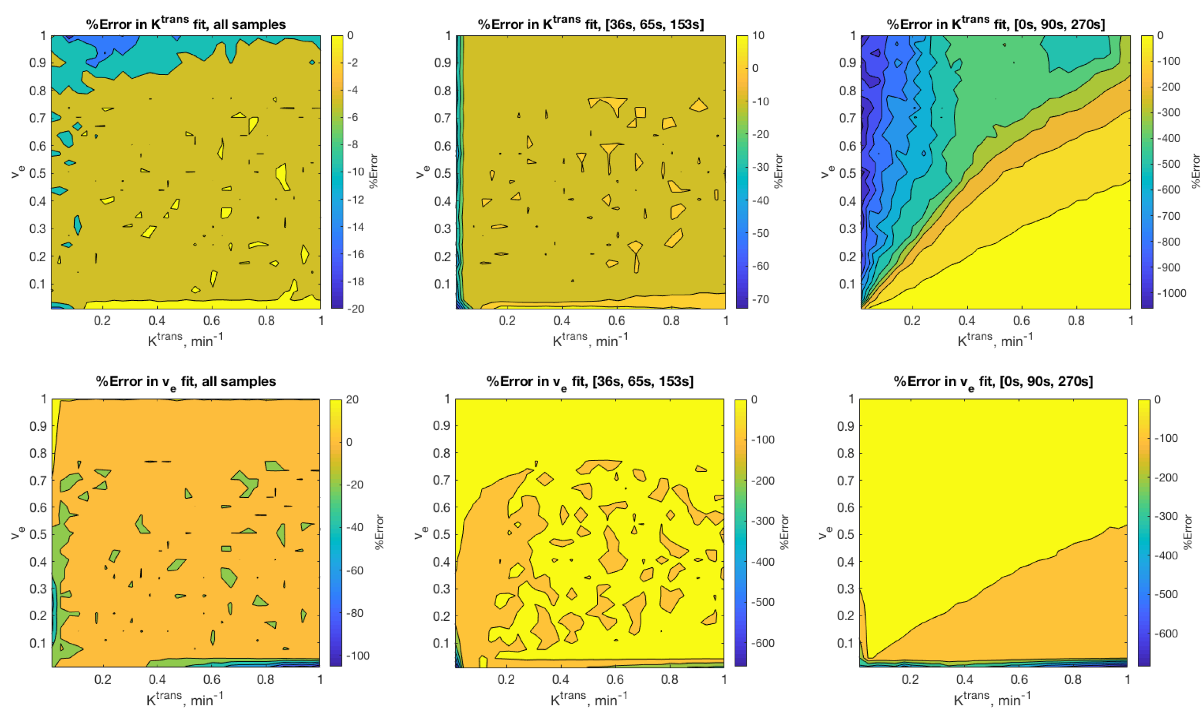
The SER three-time point fits had the largest range in average fit error across parameter values: from 1-1000% for K^trans and 0.03 to 686% for v_e. The ASC three-time point fits had the next largest range in average fit error across parameter values, from <0.01 to 73% for K^trans and <0.01 to 659% for v_e. The full-length noisy time course had the smallest range in average fit error, from < 0.01 to 20% for K^trans and <0.01 to 105% for v_e. In all sampling cases, largest errors were at the smallest values of K^trans or v_e. The contour maps in Figure 3 show how the error in fit as averaged over 500 repetitions is distributed across parameter ranges.

Discussion and Conclusion

Simulations indicate that using analysis of simplicial complexes, three-timepoint sampling can be used to estimate standard Kety-Tofts kinetic parameters. Since increasing acquisition time should result in lower noise levels, error in estimated parameters should be even more decreased than our simulations indicate. Further work will be carried out to validate the method in our current patient data set.

Acknowledgements

We gratefully acknowledge the support of NCI U01CA142565, U01CA174706, and CPRIT RR160005.