4564
Prostate cancer detection with biophysical modeling of diffusion and relaxometry1Radiology, New York University School of Medicine, New York, NY, United States, 2Microstructure Imaging INC, New York, NY, United States, 3Memorial Sloan Kettering Cancer Center, New York, NY, United States
Synopsis
For prostate cancer imaging, increasing the echo time selectively suppresses the cellular tissue, and emphasizes luminal water. We study the ADC dependence on echo time and diffusion time in 3 patients with PIRADS≥4 lesions, and propose a modeling strategy to interpret the changes in signal, as lumen diameter and volume fraction shrink during cancer progression. We evaluate cellular and luminal diffusivities, volume fractions, and luminal diameters as cancer biomarkers.
Introduction
The prostate imaging reporting and data system (PIRADS) has established a set of recommendations for characterization of prostate lesions through a multi-parametric MRI exam, which features $$$T_2$$$-weighted ($$$T_2w$$$), diffusion weighted imaging (DWI), and dynamic contrast enhanced (DCE) MRI. PIRADSv2.11 discourages long echo-times for both $$$T_2w$$$ and DWI. At long $$$T_E$$$, fast spin echo $$$T_2w$$$ images would experience spatial blurring due to the long echo-train length, while long-$$$T_E$$$ DWI would drown under the noise floor. These PIRADS recommendations were based on image quality, and did not attempt to optimize the overall contrast.Recently, using low-spatial resolution/high SNR, a non-trivial dependency of DWI on $$$T_E$$$ has been shown in volunteers. It was used to separate cellular (dominating at short $$$T_E$$$) from luminal (visible at long $$$T_E$$$) tissue compartments2. As the luminal diameter changes strongly in prostate cancer (from 300 down to 20 microns)3, we hypothesize stronger DWI contrast at longer $$$T_E$$$.
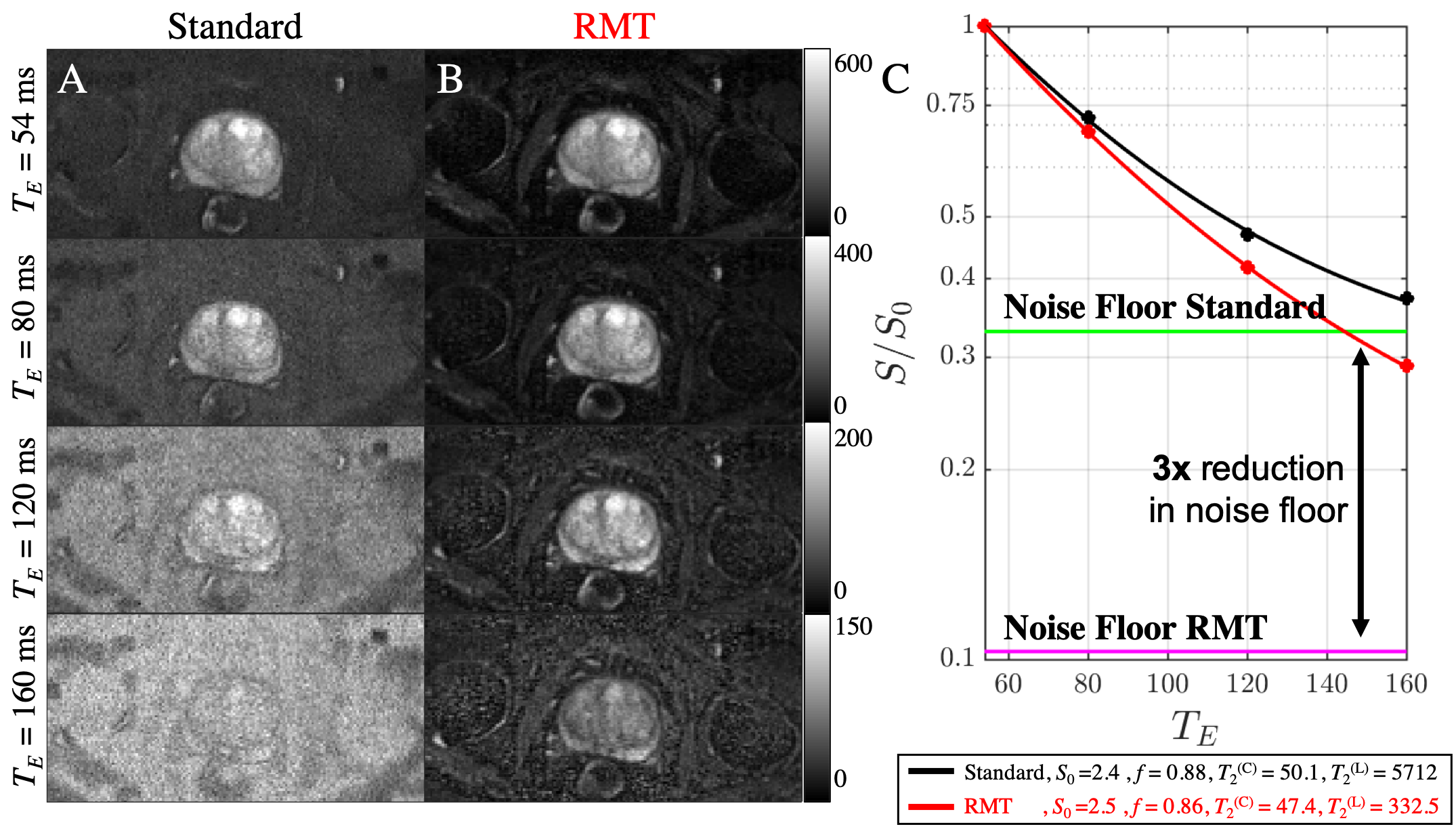
Here we use random matrix theory (RMT) reconstruction4 to increase the SNR of prostate DWI by 3-fold, for characterization of the relative contrast of the prostate MRI exam at long $$$T_E$$$.
Methods
MRI: 3 Patients with PI-RADS 4-5 transition zone lesions, underwent multi-parametric prostate MRI on a 3T scanner (GE Healthcare DiscoveryTM MR750, Waukesha, WI) with an 8-channel pelvic surface array coil. Pulsed gradient spin echo DWI EPI was acquired on 3 non-collinear gradient directions for b=50 s/mm2 and b=1000 s/mm2, with 2 and 14 averages respectively. Other imaging parameters include $$$T_R = 8$$$s, T_E = [54,80,120,160] ms, diffusion time = [23,23,46,46] ms, bandwidth = 1953.12 Hz/pixel, voxel size = 1.375x1.375x4 mm3, FOV = 220x110x108 mm3, partial Fourier = 5/8 filled with POCS, and coil images were combined via adaptive combination5. In-line averaging for both standard and RMT images was performed after PCA-based phase estimation4,6.Modeling: The apparent diffusion coefficient (ADC) and diffusion-free signal ($$$S|_{b=0}$$$) are calculated for each voxel via weighted linear least-squares7. Since our acquisition varied diffusion time together with the echo time, the ADC contrast depends on both parameters, whereas the “$$$T_2w$$$” image, only depends on $$$T_E$$$:$$S(b,T_E,t)=S|_{b=0}(T_E)\cdot e^{-b\cdot ADC(T_E,t)}$$
By leveraging the large differences in $$$T_2$$$2,8-10 between compartments and relatively high SNR, biexponential $$$T_2$$$ could be measured from $$$S|_{b=0}$$$:
$$S|_{b=0(T_E)}=S|_{b,T_E=0}\bigg(\underbrace{fe^{-T_E/T_2^{(C)}}}_C+\underbrace{(1-f)e^{-T_E/T_2^{(L)}}}_L\bigg).$$
Here $$$f$$$ is the cellular compartment fraction, $$$T_2^{(C)}$$$ and $$$T_2^{(L)}$$$ represent the fast (cellular) and slow (luminal) $$$T_2$$$ compartments. These values are then used to determine $$$T_E$$$-specific weights that define diffusion compartments of the prostate:$$ADC(T_E,t)=W(T_E)\cdot D^{(C)}(t)+(1-W(T_E))\cdot D^{(L)}(t),\,\,\,\mathrm{where}\,\,W(T_E)=\frac{C}{C+L}$$
To resolve compartment diffusivities, we introduce their time-dependent models. $$$D^{(C)}(t)$$$ is modeled by the short-time limit2,11:$$D^{(L)}(t)=D^{(L)}_0\bigg(1-\frac{4}{9\sqrt{\pi}}\frac{S}{V}\sqrt{D^{(L)}_0t}\bigg),$$where the luminal surface-to-volume ratio, $$$S/V$$$, is related to the luminal diameter, $$$\bar{a}^L=6V/S$$$. $$$D^{(C)}(t)$$$ is modeled by the extended disorder power-law2,12,13:$$D^{(C)}(t)=D_\infty^{(C)}+A\cdot t^{-1/2},$$ with finite bulk cellular diffusion constant $$$D_\infty^{(C)}$$$ and the slope $$$A$$$ of the power-law tail quantifying the combination of cellular diameters and permeability. Both $$$S|_{b=0}(T_E)$$$ and $$$ADC(T_E,t)$$$ estimations were performed using dictionary-matching approach.
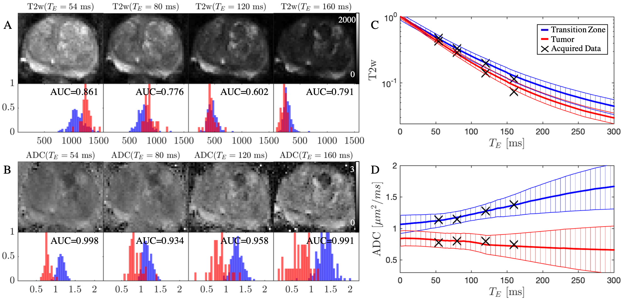
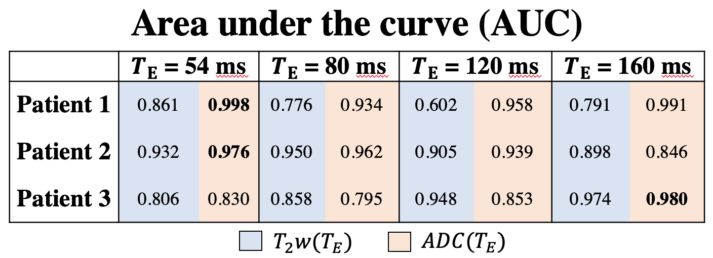
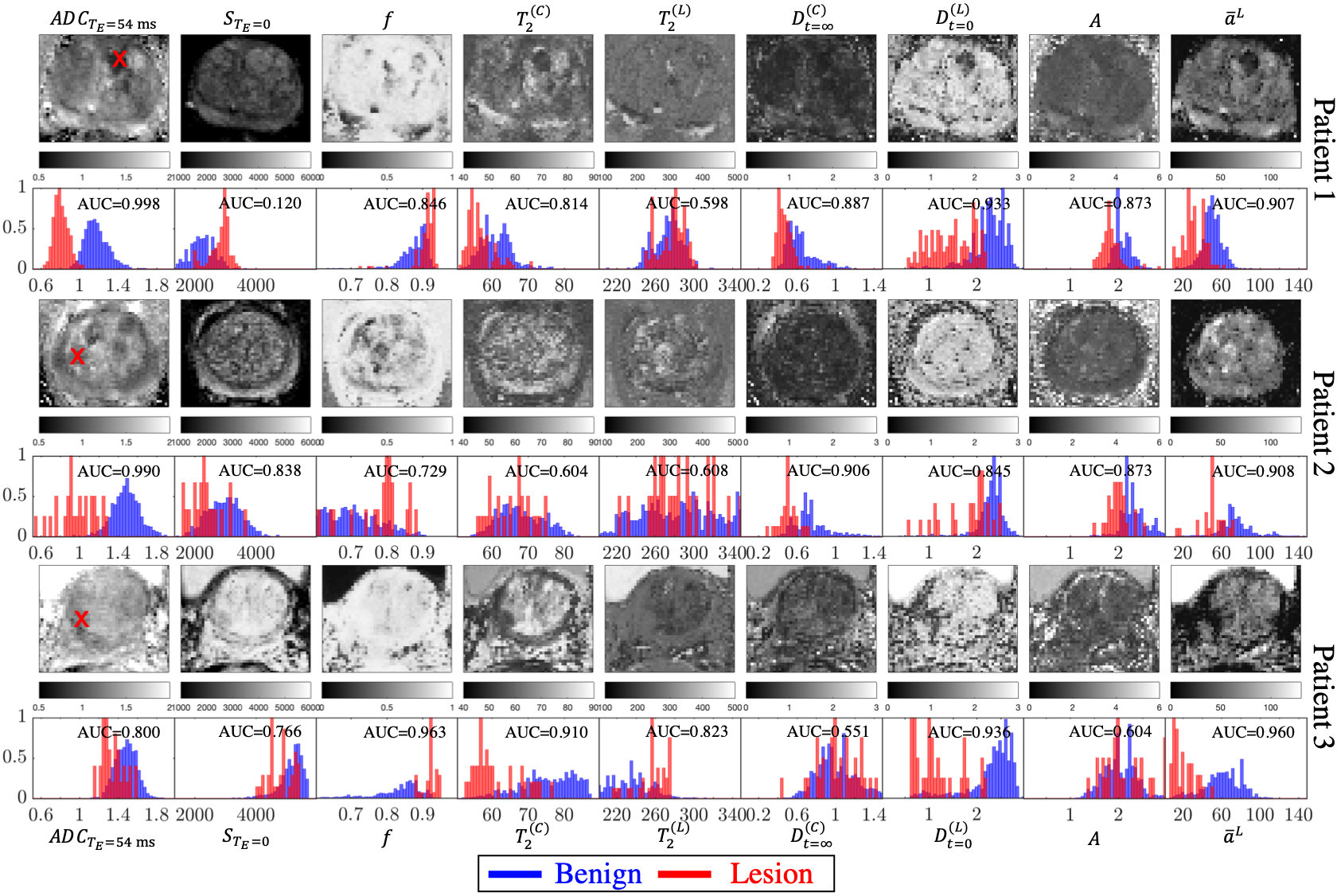
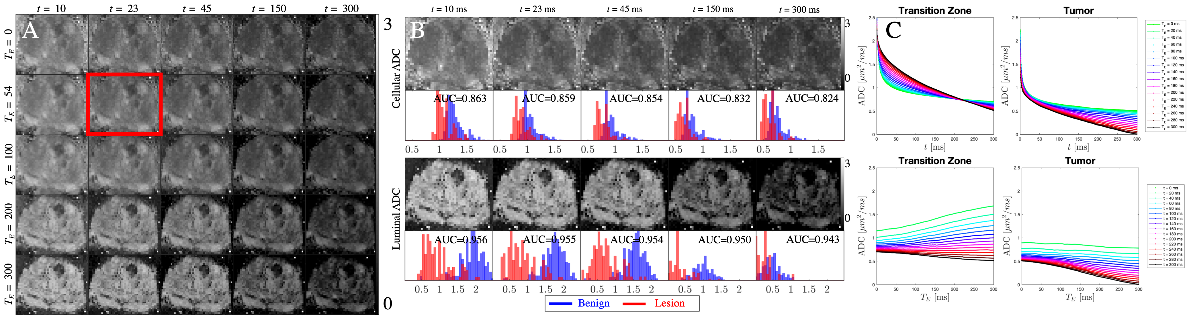
We apply this modeling approach to benign and malignant transition zones, thereby evaluating the effect of varying the echo time [Fig.2] on $$$ADC$$$ and $$$T_2w$$$ contrasts. We consider a series of synthesized $$$ADC(T_E,t$$$)-maps as potential new biomarkers [Fig.3], and demonstrate the evolution of ADC contrast with echo time for each compartment [Fig.4]. Area under the curve (AUC) analysis was used to determine the number of true positives versus false-positives between benign and lesion ROIs.
Results & Discussion
Following RMT reconstruction, there is a 3x reduction in the noise floor [Fig.1], allowing for sufficiently high SNR at long $$$T_E$$$, such that the signal is well above the noise floor [Fig.1]. Without RMT, our findings related to the long $$$T_2$$$ (luminal compartment) would be biased by the noise floor.As $$$T_E$$$ increases, $$$ADC$$$ increases in benign, but less so in malignant tissue, which can be explained by selective suppression of cellular water due to increased $$$T_2$$$ weighting [Fig.2,5]. A profound increase in $$$ADC$$$-contrast between benign and malignant tissues is observed with increasing $$$T_E$$$ [Fig.2], in line with high grade lesions having smaller luminal fractions3,10. The variation in $$$ADC$$$ also increased due to higher sensitivity to biological variation within the ROI. The corresponding AUC as function of $$$T_E$$$ (Fig.3) demonstrates an optimal $$$T_E$$$ for different patients, overall longer than currently used $$$T_E$$$ in clinic.
Furthermore, biophysical modeling provides increased granularity towards diagnosis, as the lesion shows increased $$$f$$$ and decreased (consistent with histology)3 for all three patients [Fig.4]. While the cellular volume fraction, $$$f$$$, has been proposed as a quantitative biomarker10,14,15 for prostate cancer diagnosis, our data shows that the luminal diameter changes more dramatically in malignant versus benign tissue [Fig.3,4]. The precision of these parameters and correlation with cancer grade will be determined as more patients are scanned, which is ongoing.
Conclusions
We show here that $$$T_E$$$ is a critical covariate for separating between benign and malignant tissue with $$$ADC$$$ in prostate cancer. RMT-reconstruction is crucial for exploring previously unattainable and valuable regions in the parameter space (e.g., long $$$T_E$$$). We also showcase the additional value of biophysical modeling (ref.2) based on a clinically feasible acquisition to extract the luminal diameter, which could serve as a biomarker in prostate cancer diagnosis.Acknowledgements
This work was supported by R01 EB027075 (NIBIB) and by the Center of Advanced Imaging Innovation and Research (CAI2R, www.cai2r.net), a NIBIB Biomedical Technology Resource Center: P41 EB07183.References
1. Weinreb JC, Barentsz JO, Choyke PL, et al. PI-RADS Prostate Imaging – Reporting and Data System: 2015, Version 2. European Urology 2016;69:16-40.
2. Lemberskiy G, Fieremans E, Veraart J, Deng F-M, Rosenkrantz AB, Novikov DS. Characterization of Prostate Microstructure Using Water Diffusion and NMR Relaxation. Frontiers in Physics 2018;6.
3. Gilani N, Malcolm P, Johnson G. A monte carlo study of restricted diffusion: Implications for diffusion MRI of prostate cancer. Magn Reson Med 2017;77:1671-7.
4. Lemberskiy G, Baete S, Veraart J, Shepherd TM, Fieremans E, Novikov DS. Achieving sub-mm clinical diffusion MRI resolution by removing noise during reconstruction using random matrix theory. In Proceedings 27nd Scientific Meeting #0770, International Society for Magnetic Resonance in Medicine, Montreal, Canada, 2019 2019.
5. Walsh DO, Gmitro AF, Marcellin MW. Adaptive reconstruction of phased array MR imagery. Magn Reson Med 2000;43:682-90.
6. Kordbacheh H, Seethamraju RT, Weiland E, et al. Image quality and diagnostic accuracy of complex-averaged high b value images in diffusion-weighted MRI of prostate cancer. Abdominal Radiology 2019;44:2244-53.
7. Veraart J, Sijbers J, Sunaert S, Leemans A, Jeurissen B. Weighted linear least squares estimation of diffusion MRI parameters: strengths, limitations, and pitfalls. Neuroimage 2013;81:335-46.
8. Kjaer L, Thomsen C, Iversen P, Henriksen O. In vivo estimation of relaxation processes in benign hyperplasia and carcinoma of the prostate gland by magnetic resonance imaging. Magn Reson Imaging 1987;5:23-30.
9. Gilani N, Rosenkrantz AB, Malcolm P, Johnson G. Minimization of errors in biexponential T2 measurements of the prostate. J Magn Reson Imaging 2015;42:1072-7.
10. Sabouri S, Chang SD, Savdie R, et al. Luminal Water Imaging: A New MR Imaging T2 Mapping Technique for Prostate Cancer Diagnosis. Radiology 2017;284:451-9.
11. Mitra PP, Sen PN, Schwartz LM. Short-time behavior of the diffusion coefficient as a geometrical probe of porous media. Phys Rev B Condens Matter 1993;47:8565-74.
12. Novikov DS, Fieremans E, Jensen JH, Helpern JA. Random walk with barriers. Nat Phys 2011;7:508-14.
13. Novikov DS, Jensen JH, Helpern JA, Fieremans E. Revealing mesoscopic structural universality with diffusion. Proc Natl Acad Sci U S A 2014;111:5088-93.
14. Panagiotaki E, Chan RW, Dikaios N, et al. Microstructural characterization of normal and malignant human prostate tissue with vascular, extracellular, and restricted diffusion for cytometry in tumours magnetic resonance imaging. Invest Radiol 2015;50:218-27.
15. Chatterjee A, Bourne RM, Wang S, et al. Diagnosis of Prostate Cancer with Noninvasive Estimation of Prostate Tissue Composition by Using Hybrid Multidimensional MR Imaging: A Feasibility Study. Radiology 2018;287:864-73.
16. Veraart J, Fieremans E, Novikov DS. Diffusion MRI noise mapping using random matrix theory. Magn Reson Med 2016;76:1582-93.
Figures