Introduction

Stroke, a major cause of death worldwide, is very time sensitive: the earlier its detection and treatment, the higher the recovery chances^[1]. Diffusion weighted imaging(DWI) MR sequences are recommended for ischemic stroke diagnosis, as they can detect early tissue changes, enabling to distinguish stroke lesions from healthy brain tissue^[2]. In remote world areas or across poor-income groups, the lack of accessibility to MRI has been shown to impact patient outcome (e.g.,north-east India)^[1]. A potential solution would be to create a point-of-care system using an ultra-low field(ULF) magnetic field, increasing accessibility at reduced cost. However, DWI at ULF is challenging, both due to the lower intrinsic signal and also due to the hardware constraints which limit the achievable DW contrast, i.e. B₀ field, maximum gradient amplitude(gm) and maximum slew rates(sm)^[3]. We tested different MR system configurations, investigating the impact of B₀, gm, spatial resolution and b-value on the signal-to-noise ratio(SNR) and contrast-to-noise ratio(CNR) for stroke lesion detectability.

Methods

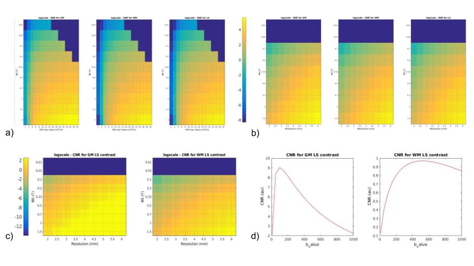
Theoretical study of SNR and CNR
To study the DWI SNR dependency across B₀ strengths, we expand the SNR tissue (Gray Matter-GM, White Matter-WM, Lesion-LS) per time unit equation for a spoiled gradient echo sequence from Marques, 2019^[4]. This equation accounts for the steady-state of the longitudinal magnetization, transverse relaxation with T₂ (as DWI is typically a spin-echo sequence), signal decay due to diffusion weighting and the impact of varying spatial resolution:

$$$SNR_{tissue}=B_0^{3/2} \frac{1}{\sqrt{TR_{Total}}} \frac{1}{\sqrt{BW}} sin(\alpha) e^{-\frac{TE}{T_{2, tissue}}}\frac{1-e^{-\frac{TR}{T1_{1, tissue}}}}{1-cos(\alpha) e^{-\frac{TR}{T_{1, tissue}}}} e^{-b <ADC>} (res_{test})^3$$$ (1)

figuring the flip angle ($$$\alpha$$$), repetition time(TR), echo time(TE), the readout bandwidth(BW) , relaxation times(T₁,T₂), mean tissue diffusivity(<ADC>), b-value(b) and tested spatial resolutions(res_test). The first term reflects the power law dependence on B₀ of the intrinsic signal; relaxation times were set depending on B₀ according to^[4], was the Ernt angle considering the minimum TR required for whole brain coverage (number of slices varied with resolution), and TE and bandwidth were calculated depending on gm and the desired b-value. As diffusion sequences are very sensitive to motion, the k-space is most often sampled following a single excitation. The most used sequence in clinical scanners is Echo Planar Imaging(EPI)^[5]; however spiral readouts have the advantage of starting at the center of the k-space and to enable a more efficient usage of the gradients, particularly important in slew-rate limited conditions^[6]. Both types of readouts were considered, and the following combinations for B0=[0.01 0.05 0.1 0.2 0.3 0.5 0.7 1 1.5 3](T); gm= [0.001:0.002:0.030](T/m), for lower values of B0 some gm were omitted; b=[10 50:50:1000](s/mm²) and res=[2:0.5:6](mm), were tested and the expected SNR and CNR determined. The CNR value was the difference between two SNR_tissue values among WM and LS. All SNR values were referenced to a realistic WM SNR value (40 for a non-DW image) at clinical scanner conditions (B0=1.5T, gm=0.03T/m, b=1000s/mm²).

Image Simulation
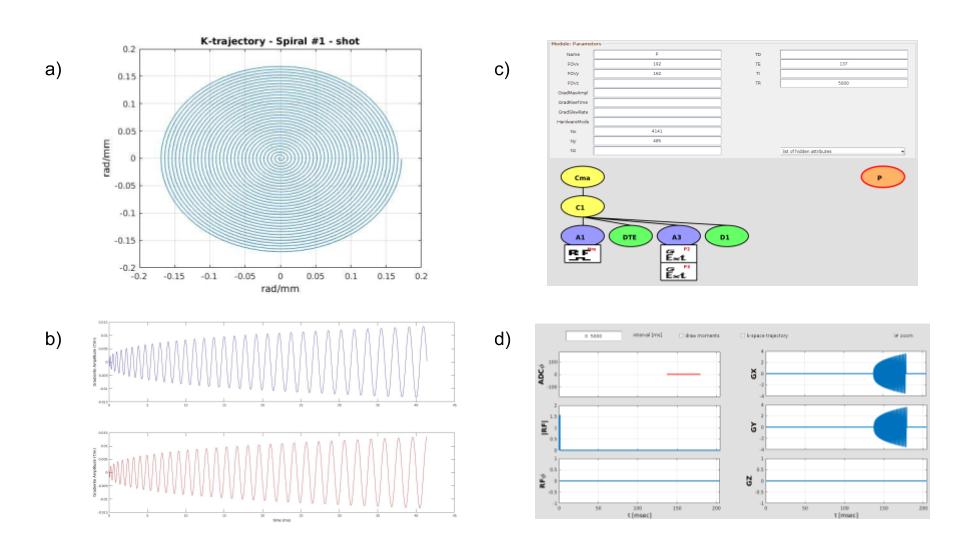
For illustration purposes, we considered four possible MR system scenarios and simulated brain images for the theoretically determined SNR for each specific tissue region. Matlab^® was used to create the sequence to feed to the JEMRIS simulator^[7]-Fig.1, the brain sample was modified to account for relaxation times at each B0 strength. K-space data was generated for each tissue type, and attenuated according to its diffusivity (mm2/s) (<ADC>CSF,GM,LS=3.2x10-3,8.0x10-4,7.0x10-4,5.5x10-4)^[8][9] noise was then added according to the theoretical study results. Data was reconstructed using Gridding (see https://github.com/wandell/mrTutorials-matlab) (kernel_width=3, with Voronoi density pre- and pos-compensation), followed by application of the Fast Fourier Transform.

Results

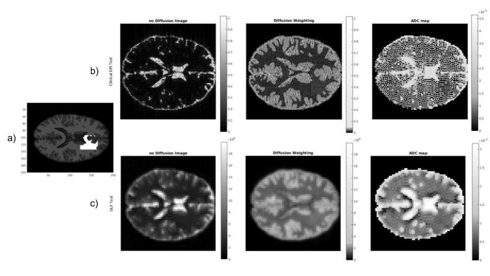
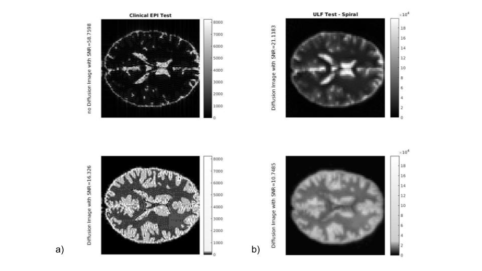
As expected, the lower the B0and gm values, the poorer SNR/CNR performance - Fig. 2. For a set of B0 and gm, a possible b-value of 400 s/mm2 creates a maximum relative in terms of CNR between WM and LS, and also resolution push both the SNR/CNR up. SPIRAL always outperforms EPI in terms of SNR/CNR- Fig 3. The simulated brain images are shown in Fig 4. for both a clinical setting (1.5T) and a ULF MR system. The LS tissue is slightly visible in both implementation. Fig 5 depicts the added noise in the reconstructed image, where is depicted higher values mean SNR for WM mask in EPI sequence, even though there is a tissue sensitivity even with the Spiral ULF system sequence.

Discussion

ULF MR systems constraints reduce, as expected, the SNR/CNR, but sacrificing resolution can mitigate the loss. Mainly due to its lower TE and shorter readout times, the spiral sequence outperforms EPI. Here we are ignoring that artifacts due to B0 inhomogeneity and non-ideal gradients tend to be more benign in EPI, which is why spiral readouts are not typically used. However, accurate B0 and gradient mapping have been shown to enable good quality spiral DW imaging [10].Improvements in SNR using super-resolution reconstruction and denoising (possibly with deep learning) should be considered in the future [11].

Conclusion

IULF MR scanners show potential for point-of-care stroke diagnostics and experimental work on this research area should continue to be pursued.

Acknowledgements

This work was supported by Department of Science and Technology under an Indo-Portugal Grant, Development of low field MRI scanner for stroke imaging, Int/Portugal/P-09 /2017 and Fundação para a Ciência e a Tecnologia, Portugal.