4503
NODDInet: Diffusion parameter mapping using deep neural network trained by computer simulation data1Seoul National University, Korea, Republic of Korea
Synopsis
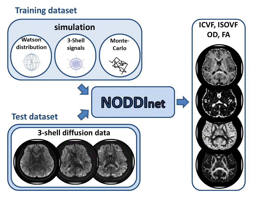
A deep neural network, NODDInet, was developed to generate NODDI parameters (ICVF, ISOVF, OD, and FA) in 1 min. This network was trained using a computer simulation-generated training dataset only, and, therefore, is unbiased to experimental data and covers a wide range of the parameters. For the network input, the diffusion measurements of each shell were projected onto three 2D plains to reduce the input data size while preserving the geometric information of the diffusion measurements. The results demonstrate higher accuracy and faster processing time (x14) than a previous method (AMICO).
Introduction
Neurite orientation dispersion and density imaging1 (NODDI) utilizes multi-shell diffusion data to estimate neurite density and dispersion parameters and has been widely used. However, the method requires extremely long computation time, taking 17 hours for one dataset. To shorten the processing time, AMICO2 (processing time: ~16 min) was developed at the cost of increased errors. In this study, we developed a deep neural network to generate NODDI parameters (intra-cellular volume fraction (ICVF) isotropic volume fraction (ISOVF), orientation dispersion (OD), and fractional anisotropy (FA)) in 1 min. This network was trained using a computer simulation-generated training dataset only, and, therefore, is unbiased to experimental data and cover a wide range of the NODDI parameters. Furthermore, we designed a new approach of generating a network input dataset that retains the geometric information of the multi-shell diffusion measurements while reducing input size. The results demonstrate higher accuracy and faster processing time (x14) than AMICO.Methods
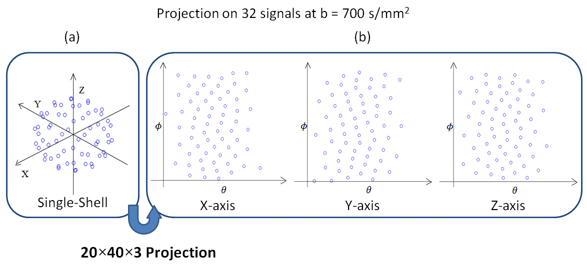
[Diffusion simulation] The training dataset for the network was generated by a Monte-Carlo computer simulation. A total of 17000 microstructural environments were generated to cover a wide range of the parameters in NODDI. The environment assumed three pools, intra-cellular, extra-cellular, and CSF, and the volume fraction of each pool was determined by ICVF (between 0 to 1) and ISOVF (between 0 to 1). Once the volume fraction was determined, 2×10⁵ protons were assigned to each pool by their volume fractions. Protons in CSF performed isotropic diffusion (3.0×10⁻³ mm2s-1) whereas protons in the extra-cellular space performed anisotropic diffusion$$${d'_∥}$$$ = $$$d_{∥}$$$ - $$$d_{∥}$$$ICVF$$$\left(1-{\tau }_1\right)$$$, and $$${d'_⊥}=\ d_{∥\ }-d_{∥\ }ICVF(\left({1+\tau }_1\right)/2)$$$ where $$$d_{\parallel }$$$ = 1.7$$$\mathrm{\times}$$$10$$${}^{-3\ }$$$mm$$${}^{2}$$$s$$${}^{-1}$$$.3 Finally, protons in the intra-cellular space performed hindered diffusion along the axon vectors whose mean direction was randomly chosen. The axon vectors were dispersed by Watson distribution3. For the acquisition, the scan parameters were Δ = 46 ms, δ = 33 ms and G = 10.483, 16.031, and 27.032 mT/m for b = 300, 700, and 2000 s/mm2, respectively. For b = 300, 700, and 2000 s/mm2, 8, 32, and 64 diffusion directions were applied, respectively. Gaussian noise was added to generate SNR of 50. In total, 108 (= 8+32+64) diffusion measurements were obtained by the computer simulation for the 17000 microstructural environments.[Projection of 3D multi-shell data] The 108 diffusion measurements are sparsely located in a 3D space (Fig. 2a). If this 3D space is directly inputted to a convolutional neural network (CNN), the input size can be large, making CNN less efficient. Alternatively, one might suggest using 108x1 vector as the input for CNN. However, this vector loses geometric information of the 3D multi-shell diffusion data. In order to retain the geometric information while reducing the input data size, we projected the diffusion measurements of each shell onto three 2D plains. Each plain corresponded to a reference axis (i.e., x-, y-, and z-axis) and the position on the plain was determined by the spherical coordinate (Θ,Φ) with respectively the reference axis (Figure 2). Then each plain was resampled to generate a 20×40 matrix. Hence, a 20×40×9 matrix was constructed from the 3-shell data while retaining most of the information in the original 3D space. To demonstrate the importance of preserving the geometric information, we rearranged the first two dimensions of the input matrix randomly and trained another network (NODDInetrandom).
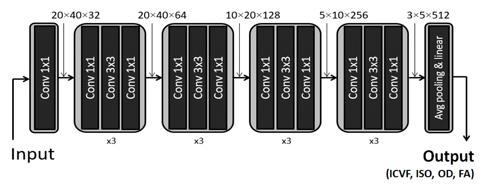
[Convolutional neural network] For the structure of NODDInet, ResNet5 was utilized (Figure 3). Using the 17000 simulated data, the network was trained to generate ICVF, ISOVF, OD, and FA. L2 loss and ADAM optimizer were used.
[Experimental data] For the evaluation of the network performance, five subjects from Ref.6 were used. The diffusion gradient amplitudes and directions were the same as in the simulation.
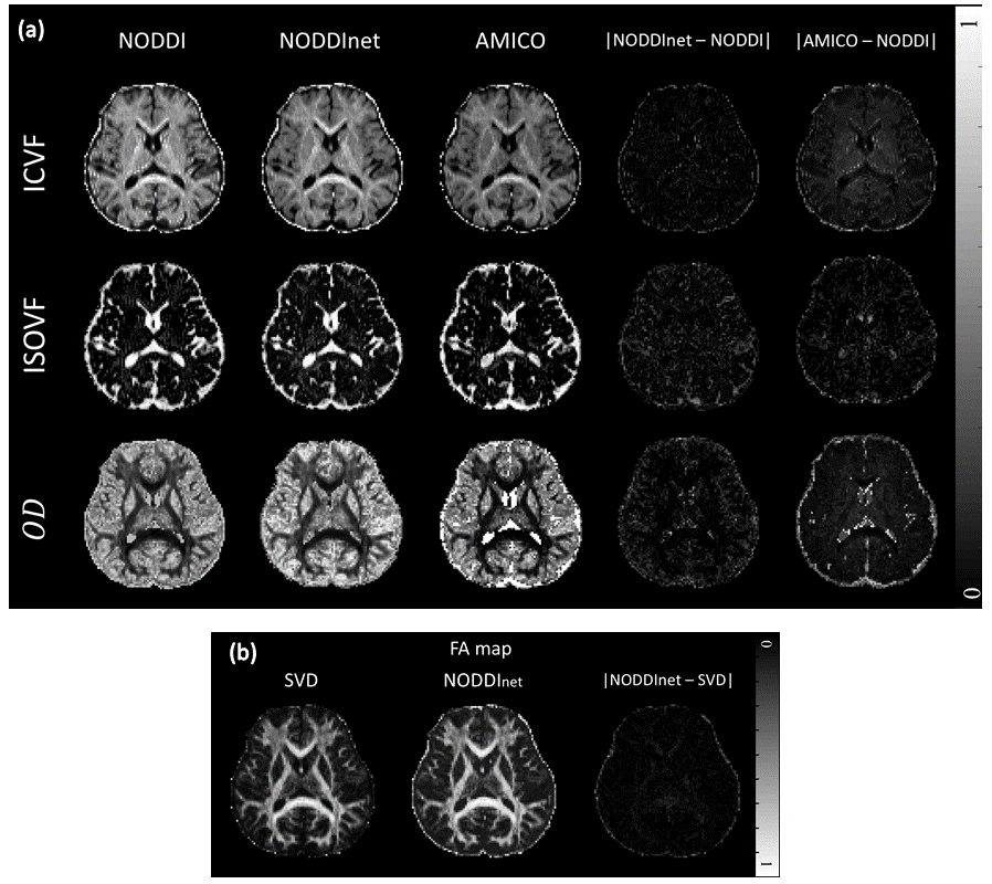
[Evaluation] The experimental data were processed with the four methods: NODDI, NODDInet, NODDInetrandom, and AMICO. Normalized root-mean-squared error (NRMSE), structural similarity (SSIM), and correlation coefficient were calculated with the NODDI results as a reference. An FA map was calculated using FSL for b = 2000 s/mm2 data and the result was compared to the FA map of the network.
Results
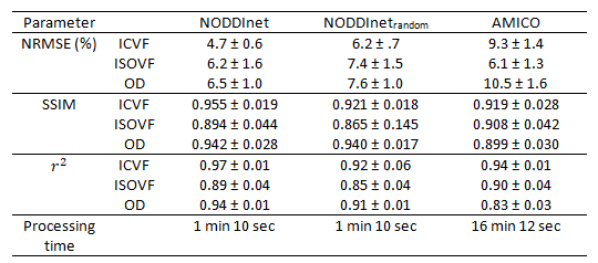
Figure 4 shows the ICVF, ISOVF, and OD maps of the three methods and the FA maps. All maps show similar contrasts. The network results are closer to those of NODDI when compared to the results of AMICO. The same trends can be found in Figure 5, which summarized the NRMSE, SSIM, and correlation coefficients. NODDInetrandom shows lower performance, demonstrating the importance of preserving the geometric information. The processing times of NODDI, NODDInet, and AMICO were 17 hours, 1 min 10 sec, and 16 min 12 sec, respectively. Hence, NODDInet is 874 times faster than NODDI, and 14 times faster than AMICO, while providing higher accuracy than AMICO.Conclusion & Discussion
In this study, NODDInet was developed. This new network showed better performances than AMICO in both accuracy and speed. The newly proposed projection idea helped to retain the geometric information, which helped to improve accuracy. NODDInet was trained by computer simulation data, and, therefore, is not biased when compared to the microstructural environments of the in-vivo data. This may help the network to be generalized for unseen experimental data.Acknowledgements
This research was supported by the National Research Foundation of Korea(NRF) funded by the MSIT(NRF-2018R1A4A1025891) and by the Brain Korea 21 Plus Project in 2019.References
[1] Zhang H, Schneider T, Wheeler-Kingshott C.A, Alexander D.C. NODDI: Practical in vivo neurite orientation dispersion and density imaging of the human brain. NeuroImage. 2019;61: 1000-1016
[2] Daducci A, Canales-Rodríguez E.J, Zhang H, Dyrby T.B, Alexander D.C, Thiran J.P, Accelerated microstructure imaging via convex optimization (AMICO) from diffusion MRI data. NeuroImage. 2015;105: 32–44.
[3] Zhang H, Hubbard P.L, Parker, G.J, Alexander, D.C. Axon diameter mapping in the presence of orientation dispersion with diffusion MRI. Neuroimage. 2011; 56 (3), 1301–1315.
[4] Liu C, Bammer R, Moseley ME. Limitations of apparent diffusion coefficient‐based models in characterizing non‐gaussian diffusion. Magnetic Resonance in Medicine. 2005;54: 419– 428.
[5] He K, Zhang X, Ren S, Sun J. Deep Residual Learning for Image Recognition. CVPR. 2016, pp. 770-778
[6] Jung W, Lee J, Shin H.G, et al. Whole brain g-ratio mapping using myelin water imaging (MWI) and neurite orientation dispersion and density imaging (NODDI). NeuroImage. 2018;182;379-388.
Figures