Introduction

Transcranial electrical stimulation (TES) methods hold promise for non-invasive therapy for conditions such as depression and epilepsy ^1,2. Improved targeting of specific neural regions will make these treatments more accurate and patient specific and improve understanding of neuromodulation mechanisms ¹. It is important to use realistic head models to simulate neural excitability caused by TES fields. Most existing research on neural activation during TES uses parallel axon geometries such as the MRG axon ^3,4. However, nerve-fiber activation also depends on nerve orientation and trajectory relative to TES electric fields ^5-7. The trigeminal nerve is a sensory motor nerve which provides tactile, proprioceptive, and nociceptive afference to the face and mouth. Neuromodulation of the trigeminal nerve can be achieved using TES ⁸. In this study we determined neural activation thresholds in a realistic trigeminal nerve geometry, measured using DTI-based tractography, compared to those in an otherwise identical straight axon to investigate the magnitude of neural activation differences caused by geometric variation.

Methods

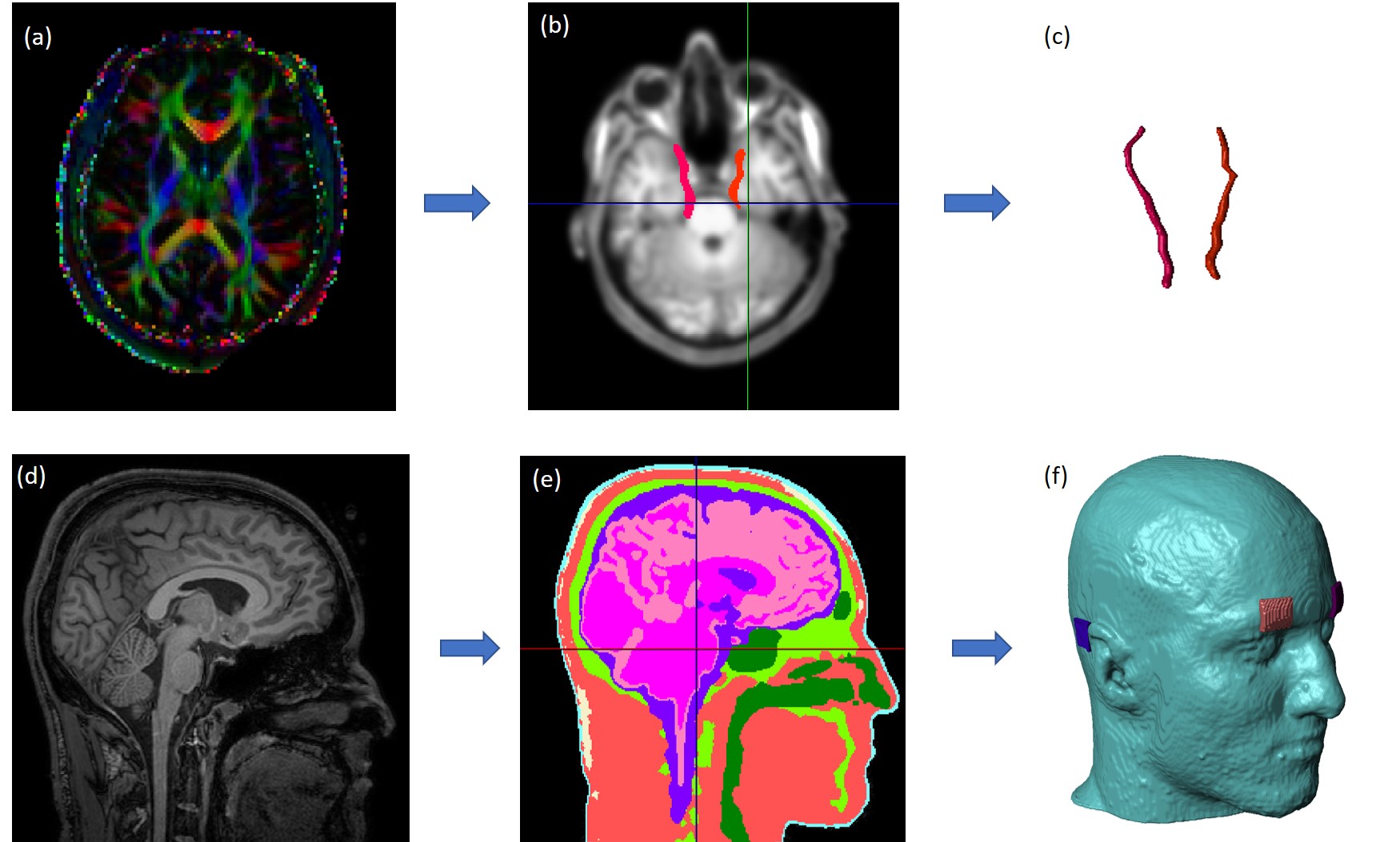
A high-resolution 3D FLASH T1-weighted structural image was acquired in a 3T MRI scanner (Philips Ingenia System, Barrow Neurological Institute, Phoenix, USA) with a 240 mm (FH) x 240 mm (AP) x 200 mm (RL) field-of-view (FOV) and 1 mm³ isotropic resolution. HARDI (high angular resolution diffusion imaging) protocol ⁹ was followed for diffusion weighted MR (DWI) data acquisition. All procedures were performed according to protocols approved by the Arizona State University Institutional Review Board. The ophthalmic and maxillary branches of the trigeminal nerve were tracked using waypoint masks and tractography methods discussed in ¹³ (Fig. 1).

Structural MR images were segmented into different tissue types using SPM12 (Wellcome Centre for Human Neuroimaging) and Simpleware ScanIP (Synopsys Inc.) to construct a labeled volume model with FOV 256 x 256 x 256 mm³, using methods outlined in ^{9, 10}. The right trigeminal nerve tract was added to the segmented model as an additional compartment. Electrodes placed at right supraorbital (RS) and mastoid process locations used for TES stimulation were also modelled (Fig. 1) and electrical properties of tissues were assigned from the literature ¹¹. The segmented labeled volume was then meshed and imported into COMSOL Multiphysics (Burlington, MA, USA). Transcranial direct current stimulation was modelled using the Laplace equation with 1mA current injection applied to the RS electrode and the other electrode grounded. The computational model had 560,732 tetrahedra and took about three hours to solve. The resulting voltages and electric field gradients were exported into MATLAB (MathWorks Inc.) as three-dimensional data of 2 x 2 x 4 mm³ voxel size.

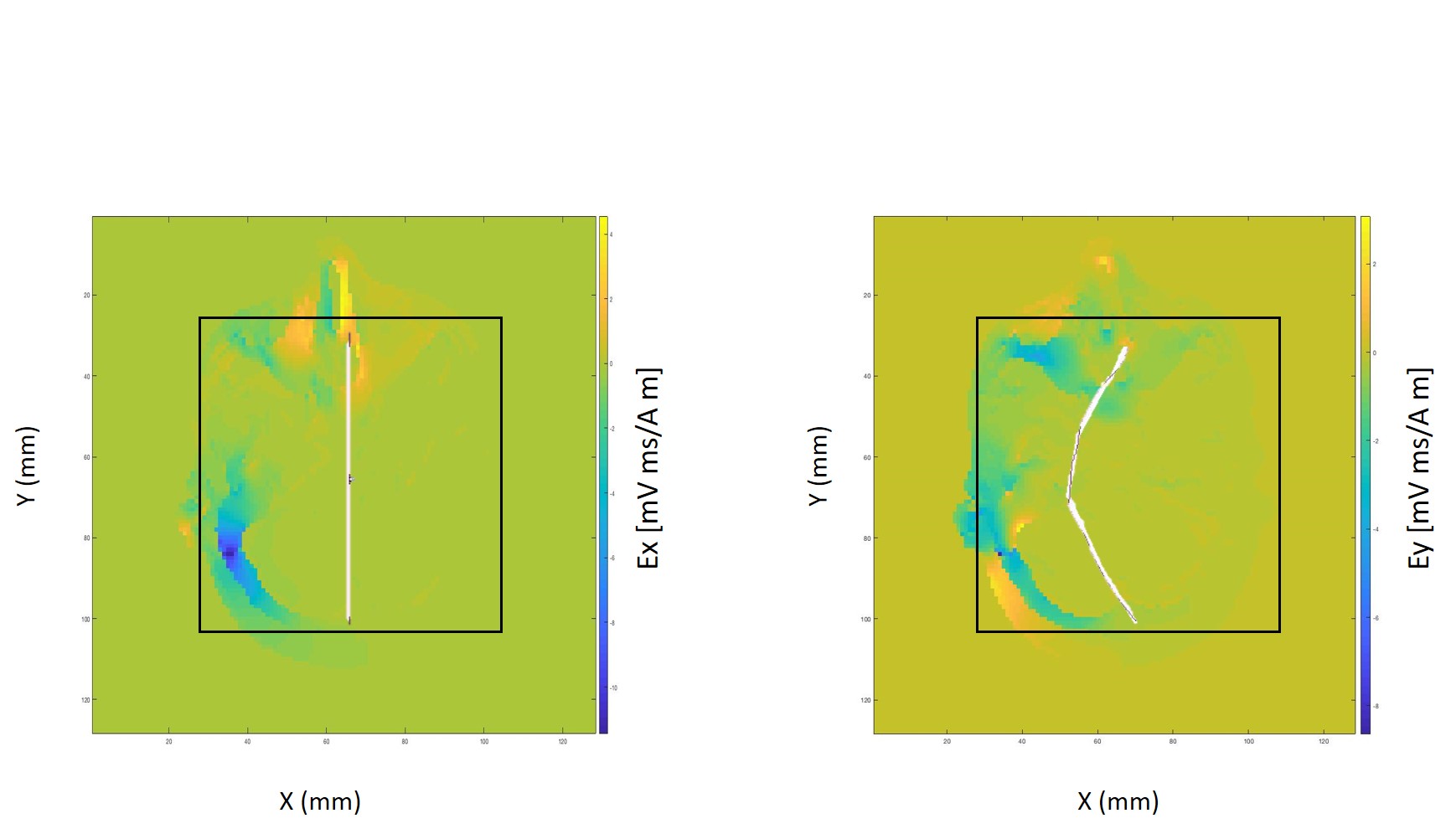
Two three-dimensional axon models were defined and solved using NEURON (neuron.yale.edu). One axon was linear, and the other followed the exact trajectory found from DTI tractography, including curves and bends. Both axons had an approximate length of 16 cm along the x direction (AP) and were assigned diameters of 2 𝞵m, cytoplasmic resistivity of 35.4 ohm-cm and homogenously distributed Hodgkin-Huxley channels ⁷. Both axons had the same number of segments, and transmembrane voltages were computed along the axon length. The resting potential was set at -65 mV. A single slice of transverse electric field (128 x 128 matrix size) was chosen from MATLAB which corresponded to axon location on FEM model (Fig. 2). On this slice an ROI of 80 x 80 matrix size was selected around the axon and interpolated to a matrix size of 160000 x 160000 𝞵m with a spatial resolution of 1 𝞵m (Fig. 2). This electric field information was multiplied by a square temporal waveform and provided as input to each axon model and its amplitude and stimulation duration were varied. The cable equation ^{3, 7, 12} was solved for both axons to obtain spatial and temporal transmembrane potentials and strength-duration graphs normalized to rheobases were plotted.

Results and Discussion

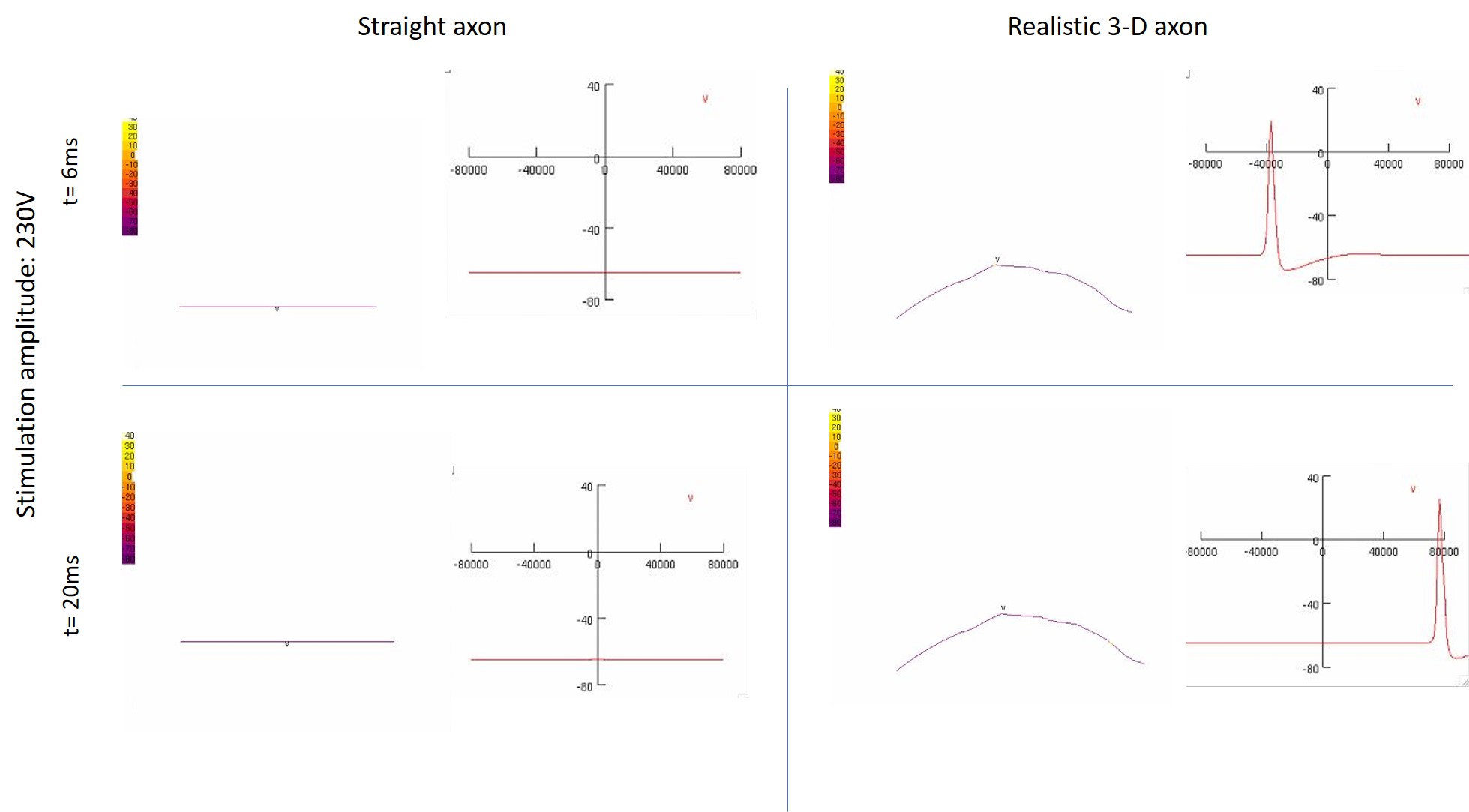
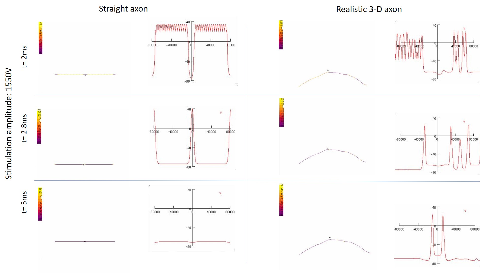
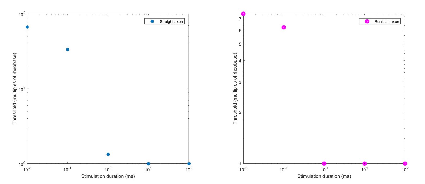
The realistic axon model predicted lower thresholds than the straight axon model. The distribution of transmembrane potential also varied along the nerve in the realistic trajectory, with differences observed along curves and bends (Figs. 3,4). This shows that the realistic axon is sensitive to the direction of the electric field with respect to the trajectory. The strength–duration curve for the realistic axon also showed smaller threshold magnitudes with a rheobase of 4000V as opposed to straight axon rheobase of 30000V (Fig. 5). Observation of clear activation differences between both axon models shows the importance of using realistic trajectories for neural excitability simulations. Future NEURON models will be made more realistic by inclusion of all physiological properties of sensory and motor axons [4] and using electric field inputs over more slices and including Ez components. Axons will be bundled to mimic a real nerve fiber and activation across various diameters will be compared.

Conclusion

Most models studying neural activation use simple geometrical neuron representations. We have shown differences in action potential patterns using a DTI-derived realistic axon compared to a straight axon. This establishes grounds for the use of realistic axon geometries for better determination of effects of three-dimensional electric fields on activity. Realistic axon models will further be used to study neuromodulation caused during TES and predict peripheral nerve stimulation caused by MR methods such as MREIT.

Acknowledgements

This study was supported by NIH award RF1MH114290 to RJS.