4435
Power-Law Behaviour of the Diffusion-Weighted Signal Under Different B-Tensor Encoding Schemes1Cardiff University Brain Research Imaging Centre (CUBRIC), School of Psychology, Cardiff University, Cardiff, United Kingdom, 2Laboratorio de Procesado de Imagen, ETSI Telecomunicacion Edificio de las Nuevas Tecnologias, Campus Miguel Delibes s/n, Universidad de Valladolid, Valladolid, Spain, 3Mary MacKillop Institute for Health Research, Faculty of Health Sciences, Australian Catholic University, Melbourne, Victoria, Australia
Synopsis
It has been shown previously that for the linear (LTE), as well as planar tensor encoding (PTE) and in tissue with 'stick-like' geometry, the diffusion-weighted signal at high b-values follows a power-law. Specifically, the signal decays as $$$1/\sqrt{b}$$$ in LTE and $$$1/b$$$ in PTE. Here, we investigate whether power-law behaviors occur with other encodings and geometries. The results show that using an axisymmetric b-tensor a power-law only exists for stick-like geometries, using LTE and PTE. Finally, using ultra-strong gradients, we confirm –for the first time in vivo– that a power-law exists for PTE in white matter of the human brain.
INTRODUCTION
Diffusion MRI probes brain microstructure based on the Brownian motion of water molecules1,2. It has been shown previously that there is a power-law relationship between the diffusion-weighted signal and the b-value at high b-values3-5. Here we investigate the effect of different b-tensor encodings6 on the diffusion-weighted signal at high b-values, including linear tensor encoding (LTE) and planar tensor encoding (PTE).Our motivation is: i) to disambiguate stick-like from other geometries (LTE shows a power-law not just for stick-like geometries, but also when there is a small contribution from dot and sphere compartments); ii) to find the range of b-values over which we observe a power-law scaling; and iii) to investigate if the signal amplitude in that range of b-value (7,000<b<10,000 $$$s/mm^2$$$) is significantly higher than the noise floor.
METHODS
In multi-dimensional diffusion MRI, the b-matrix is defined as, $$$B=b/3(1-b_\Delta)I_3+b b_\Delta\mathbf{g} \mathbf{g}^T$$$, where $$$\mathbf{g}$$$ is the diffusion gradient direction, $$$I_3$$$ is the identity matrix and the b-value, $$$b$$$, is the trace of the b-matrix. For LTE, PTE, and STE, $$$b_\Delta=1, -1/2$$$, and $$$0$$$ respectively6. The direction-averaged diffusion signal is (Eq. (34) in7):$$S(b)=\frac{\sqrt{\pi} e^{-\frac{b}{3}(D^{\mid\mid}+2D^\perp-b_\Delta(D^{\mid\mid}- D^\perp))}\textrm{erf}(\sqrt{bb_\Delta(D^{\mid\mid}-D^\perp)})}{2\sqrt{b b_\Delta(D^{\mid\mid}-D^\perp)}} \quad (1)$$
where $$$S$$$ is the normalized diffusion signal and $$$D^{\mid\mid}$$$ and $$$D^\perp$$$ are the parallel and perpendicular diffusivities respectively.
In PTE, $$$b_\Delta = -1/2$$$ and therefore:
$$S_{ic}^{PTE}(b) = \frac{\sqrt{\pi}e^{\frac{-b {D_a}^{\mid \mid} }{2}}\textrm{erfi}(\sqrt {b {D_a}^{\mid \mid}/2})}{2\sqrt{b {D_a}^{\mid \mid}/2}} \quad (2)$$
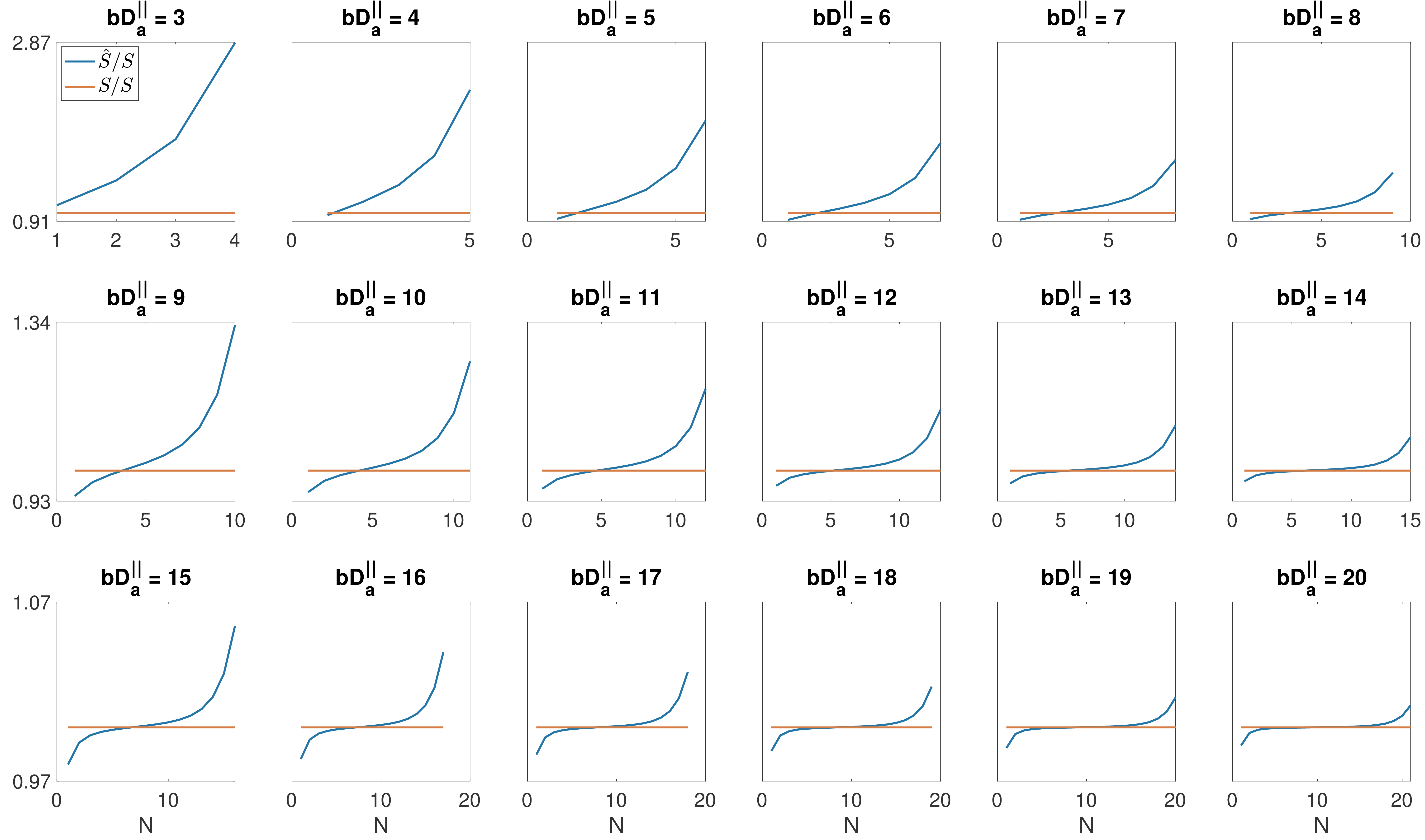
For large b-values, $$$b {D_a}^{\mid \mid} \gg 1$$$, the diffusion signal can be approximated by: $$S_{ic}^{PTE}(b) \approx \frac{1}{b {D_a}^{\mid \mid}} \sum_{k = 0}^{N} \frac{(2k-1){!}{!}}{(b {D_a}^{\mid \mid})^k} \quad (3)$$
where $$${!}{!}$$$ denotes the double factorial and N depends on the $$$b {D_a}^{\mid \mid}$$$ value (Fig. 1). A normalized error is used to compare the original, $$$S$$$ (Eq. (2)) and the approximated signal, $$$\hat{S}$$$ (Eq. (3)):
$$\textrm{Normalized error}=\frac{|S-\hat{S}|}{S} = \left|1-\frac{\hat{S}}{S}\right|\quad(4)$$
Synthetic data were generated with 60 gradient orientations8,9 and 21 b-values spaced in the interval [0, 10000 $$$s/ mm^2$$$] with a step-size of 500 $$$s/mm^2$$$. The noise is considered Rician with SNR = 150 for the b0 image10,11. A three-compartment model is used:
$$S/S_0 = f_1\int_{\mathbb{S}^2} W(\mathbf{n}) S_{cyl}(\mathbf{n}) d\mathbf{n} + f_2 \int_{\mathbb{S}^2} W(\mathbf{n}) S_{ec}(\mathbf{n}) d\mathbf{n} + f_3 S_{sph}(R_s) \quad (5)$$
where $$$f_1$$$, $$$f_2$$$, $$$f_3$$$, $$$S_{ec}$$$, $$$S_{cyl}$$$, and $$$S_{sph}$$$ are the intra-axonal, extra-axonal and the sphere signal fraction and diffusion signal12, 13 respectively, and $$$W(\mathbf{n})$$$ is the Watson ODF. The ground truth parameter values are [$$$f_1$$$ = 0.65, $$${D_a}^{\mid\mid}$$$ = 2 $$$\mu m^2 /ms$$$, $$$D_e^{\mid\mid}$$$ = 2 $$$\mu m^2 /ms$$$, $$$D_e^\perp$$$ = 0.25, 0.5, 0.75 $$$\mu m^2/ms$$$, $$$\kappa$$$ = 11, and $$$R_s = 0, 8 \mu m$$$] and axon radius $$$r_i$$$, was taken from the bins of the histograms in14 and $$$\eta = {0, 1, 1.5}$$$ are the tissue shrinkage factors14, 15.
Two healthy participants were scanned with the same protocol as the simulation. Twenty axial slices with a voxel size of $$$4 mm$$$ isotropic and a 64$$$\times$$$64 matrix size, TE = 88 ms, TR = 3000 ms were obtained.
RESULTS
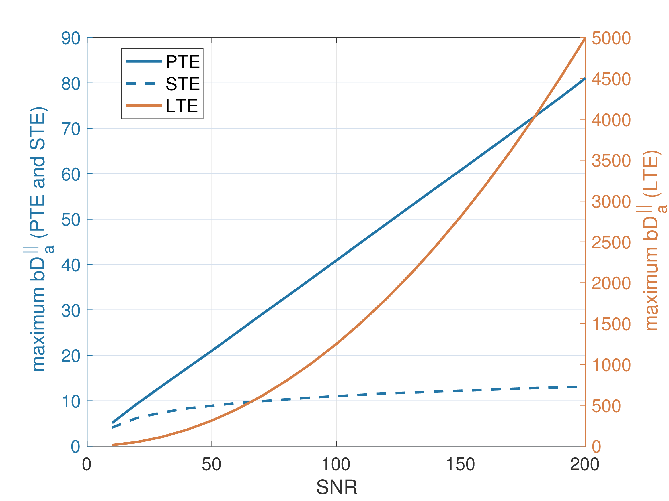
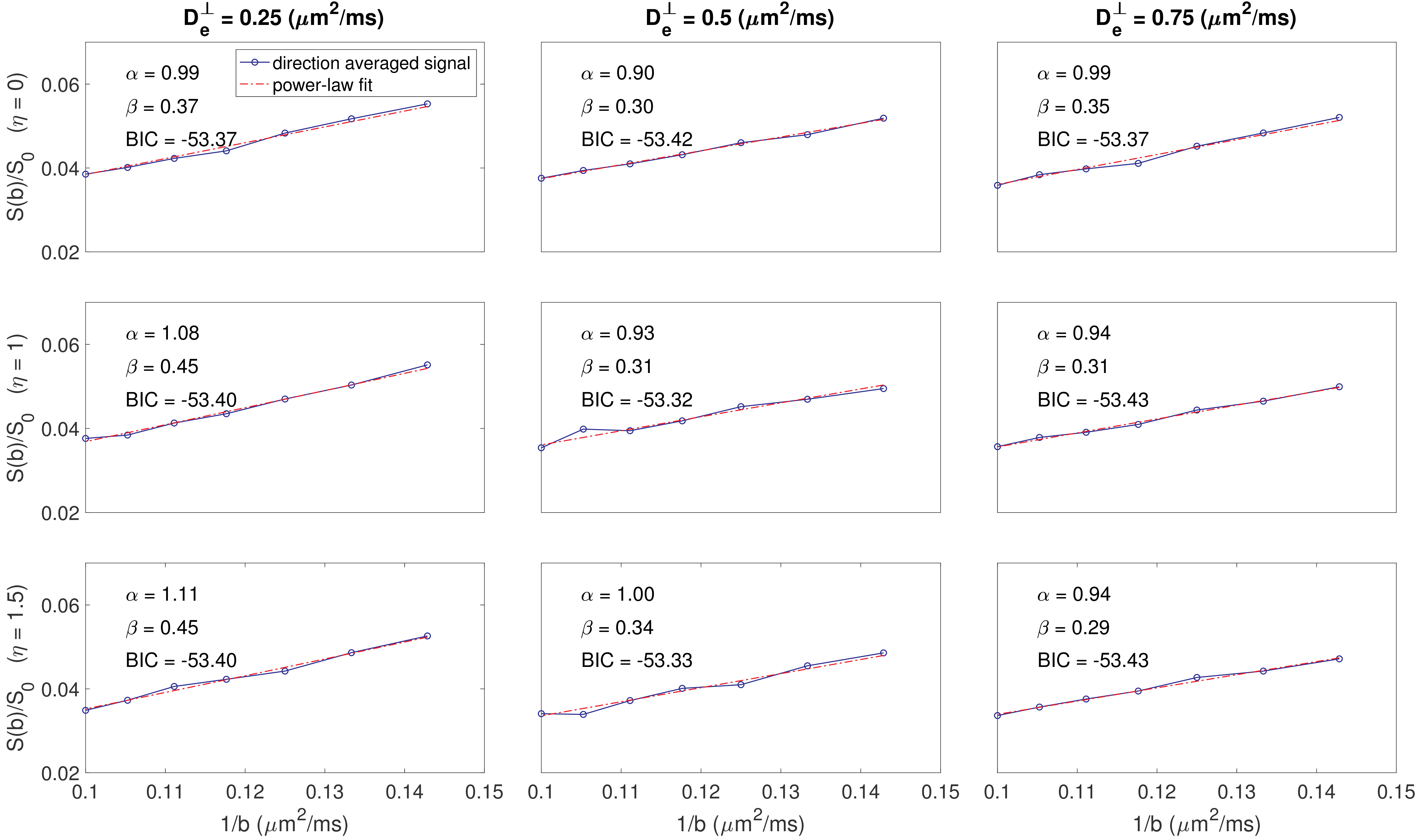
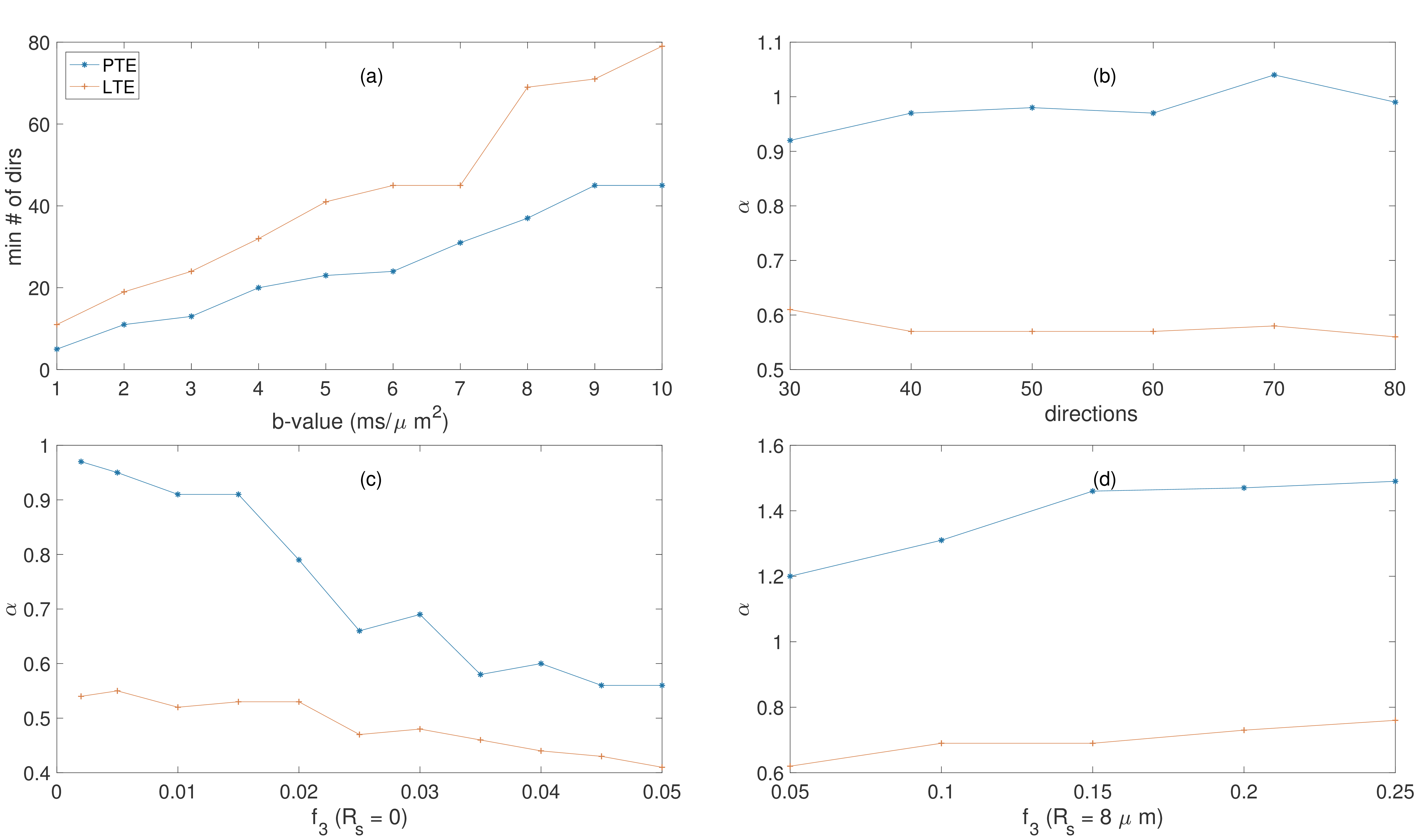
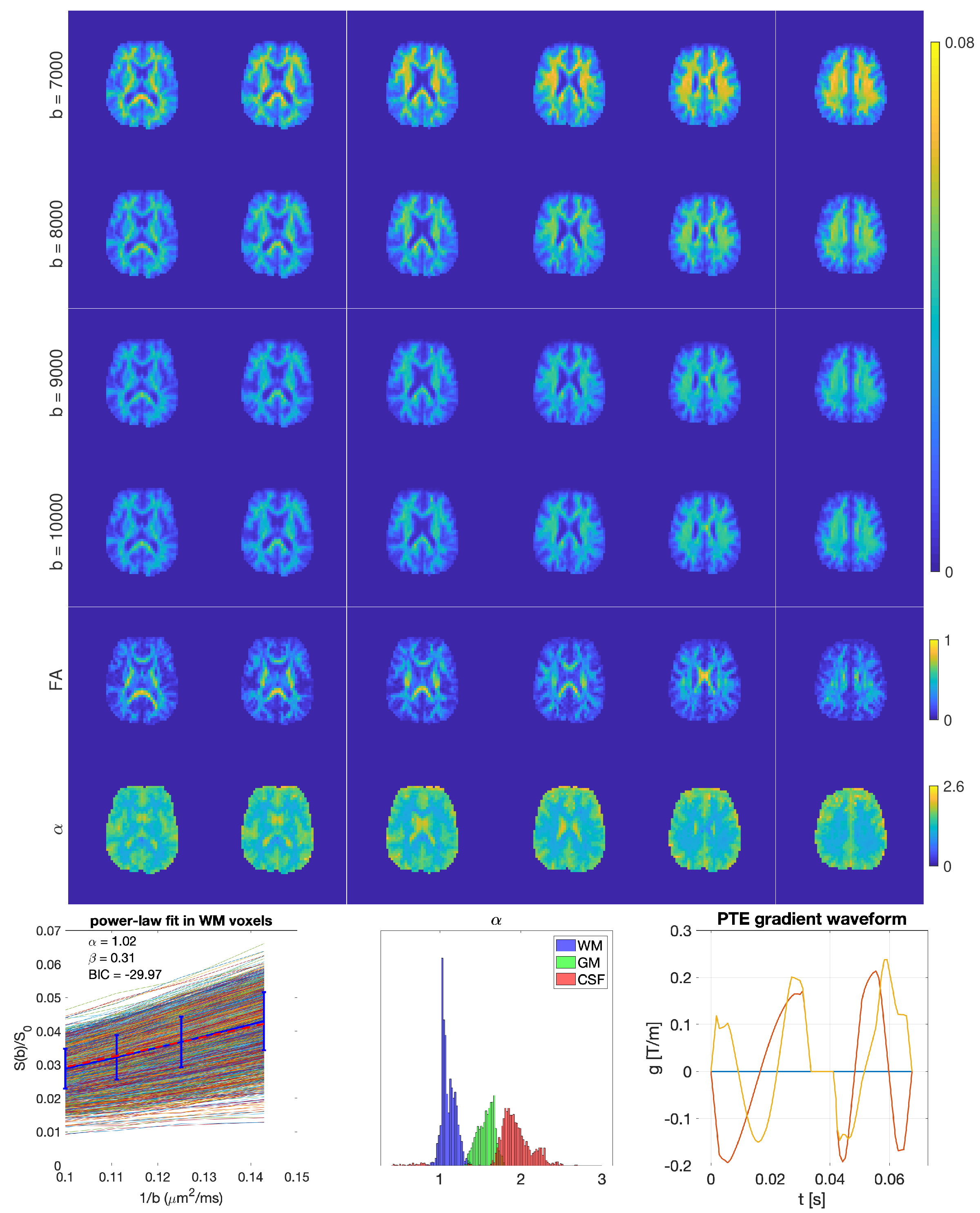
Fig. 1 shows $$$\hat{S}/{S}$$$ for $$$3<b{D_a}^{\mid\mid}<20$$$ and $$$4<N<21$$$. Fig. 2 shows the maximum $$$b{D_a}^{\mid\mid}$$$ as a function of SNR in the $$$b_0$$$ for different encoding schemes and different noise floors. Fig. 3 shows the simulated direction-averaged PTE signal ($$$f_3 = 0$$$) as a function of $$$1/b$$$ for three different perpendicular diffusivities and three different shrinkage factors. Fig. 4 shows (a) the minimum number of directions for different b-values from 1000 to 10000 $$$s/mm^2$$$ (b) the changes of exponent $$$\alpha$$$, (c) the changes of the power-law scaling, $$$\alpha$$$, versus 'still water' signal fraction, (d) the changes in the exponent $$$\alpha$$$ in the presence of spherical compartment with the radius of $$$R_s = 8 \mu m$$$ using LTE compared to PTE. Fig. 5 illustrates the normalized direction-averaged diffusion signal of the in vivo data for different b-values ($$$7000 \leq b \leq 10000$$$) in a few slices. The last three rows of Fig. 5 show the FA and $$$\alpha$$$ map, the power-law fit over white matter voxels, the histogram of the $$$\alpha$$$ values in white matter, gray matter, CSF and the PTE gradient waveform.DISCUSSION AND CONCLUSION
Our main finding here is a theoretical derivation, and confirmation in silico and, for the first time, in vivo, of a power-law relationship between the direction-averaged DWI signal and the b-value using PTE, for b-values ranging from 7000 to 10000 $$$s/mm^2$$$. In white matter, the average value of the estimated exponent is around one. For smaller b-values, this behavior must break down as the DWI signal of PTE cannot be approximated by Eq. (3) (Fig. 1) and also we cannot neglect the contribution of the extracellular compartment. It could also fail for very large b-values, if there were immobile protons that contributed a constant offset to the overall signal or if there is any sensitivity to the axon diameter16. The exponent of approximately one for white matter using PTE is consistent with the large b-value limit predicted for a model of water confined to sticks (Eq. (3)). A key finding of our work is that PTE gives a power-law if – and ONLY IF – the tissue exhibits stick-like geometry. Thus, in combination with LTE, PTE can help to disambiguate complex microstructures in vivo.Acknowledgements
The data were acquired at the UK National Facility for In Vivo MR Imaging of Human Tissue Microstructure funded by the EPSRC (grant EP/M029778/1), and The Wolfson Foundation. This work was supported by a Wellcome Trust Investigator Award (096646/Z/11/Z) and a Wellcome Trust Strategic Award (104943/Z/14/Z). S. Aja-Fernandez acknowledges the Ministerio de Ciencia e Innovacion of Spain for research grants RTI2018-094569-B-I00 and PRX18/00253 (Estancias de profesores e investigadores senior en centros extranjeros). The authors would like to thank Filip Szczepankiewicz and Markus Nilsson for providing the pulse sequences for b-tensor encoding.References
1. Callaghan PT, Eccles CD, Xia Y. NMR microscopy of dynamic displacements: k-space and q-space imaging. Journal of Physics E: Scientific Instruments. 1988 Aug;21(8):820.
2. Basser PJ, Mattiello J, LeBihan D. MR diffusion tensor spectroscopy and imaging. Biophysical journal. 1994 Jan 1;66(1):259-67.
3. McKinnon ET, Jensen JH, Glenn GR, Helpern JA. Dependence on b-value of the direction-averaged diffusion-weighted imaging signal in brain. Magnetic resonance imaging. 2017 Feb 1;36:121-7.
4. Veraart J, Fieremans E, Novikov DS. On the scaling behavior of water diffusion in human brain white matter. NeuroImage. 2019 Jan 15;185:379-87.
5. Herberthson M, Yolcu C, Knutsson H, Westin CF, Özarslan E. Orientationally-averaged diffusion-attenuated magnetic resonance signal for locally-anisotropic diffusion. Scientific reports. 2019 Mar 20;9(1):4899.
6. Topgaard D. Multidimensional diffusion MRI. Journal of Magnetic Resonance. 2017 Feb 1;275:98-113.
7. Eriksson S, Lasič S, Nilsson M, Westin CF, Topgaard D. NMR diffusion-encoding with axial symmetry and variable anisotropy: Distinguishing between prolate and oblate microscopic diffusion tensors with unknown orientation distribution. The Journal of chemical physics. 2015 Mar 14;142(10):104201.
8. Jones DK, Horsfield MA, Simmons A. Optimal strategies for measuring diffusion in anisotropic systems by magnetic resonance imaging. Magnetic Resonance in Medicine: An Official Journal of the International Society for Magnetic Resonance in Medicine. 1999 Sep;42(3):515-25.
9. Caruyer E, Lenglet C, Sapiro G, Deriche R. Design of multishell sampling schemes with uniform coverage in diffusion MRI. Magnetic resonance in medicine. 2013 Jun;69(6):1534-40.
10. Jones DK, Alexander DC, Bowtell R, Cercignani M, Dell'Acqua F, McHugh DJ, Miller KL, Palombo M, Parker GJ, Rudrapatna US, Tax CM. Microstructural imaging of the human brain with a ‘super-scanner’: 10 key advantages of ultra-strong gradients for diffusion MRI. NeuroImage. 2018 Nov 15;182:8-38.
11. Aja-Fernandez S, Vegas-Sanchez-Ferrero G. Statistical analysis of noise in MRI Switzerland: Springer International Publishing. 2016.
12. Vangelderen P, DesPres D, Vanzijl PC, Moonen CT. Evaluation of restricted diffusion in cylinders. Phosphocreatine in rabbit leg muscle. Journal of Magnetic Resonance, Series B. 1994 Mar 1;103(3):255-60.
13. de Almeida Martins JP, Topgaard D. Two-dimensional correlation of isotropic and directional diffusion using NMR. Physical review letters. 2016 Feb 23;116(8):087601.
14. Aboitiz F, Scheibel AB, Fisher RS, Zaidel E. Fiber composition of the human corpus callosum. Brain research. 1992 Dec 11;598(1-2):143-53.
15. Caminiti R, Ghaziri H, Galuske R, Hof PR, Innocenti GM. Evolution amplified processing with temporally dispersed slow neuronal connectivity in primates. Proceedings of the National Academy of Sciences. 2009 Nov 17;106(46):19551-6.
16. Veraaart J, Fieremans E, Rudrapatna U, Jones DK, Novikov DS. Breaking the power law scaling of the dMRI signal on the Connectom scanner reveals its sensitivity to axon diameters. InProceedings of the 26th Annual Meeting of ISMRM, Paris, France 2018.
Figures