Introduction

Intravoxel incoherent motion (IVIM) modeling has the potential to extract both diffusion and perfusion information from diffusion-weighted imaging data¹. The signal at low to moderate diffusion weightings can be modeled as:$$S_b/S_0=(1-f)e^{-bD}+fe^{-bD_b}F_P$$where $$$S_b/S_0$$$ is the normalized signal with b-value $$$b$$$, $$$f$$$ is the perfusion fraction, $$$D$$$ and $$$D_b$$$ are the diffusion coefficients of the extravascular space and blood respectively, and $$$F_P$$$ describes the signal attenuation in the perfusion compartment caused by diffusion encoding.
The motion of blood caused by microcirculation has been assumed to mimic a random walk^1,2, which can be characterized by a characteristic speed $$$v$$$, vessel segment length $$$l$$$ and time between direction changes $$$\tau$$$. Under this assumption the number of direction changes during diffusion encoding with duration $$$T$$$ is $$$N=T/\tau$$$.
Two important regimes have been identified^1,3: $$$N=0$$$ (ballistic regime) and $$$N\gg1$$$ (diffusive regime). Both cases provide simple analytical models, where the diffusive-regime model is by far the most commonly used. However, studies have shown that $$$\tau\sim100$$$ms, which is longer than typical encoding times^2,4, i.e. $$$N<1$$$. Also, due to the limited gradient strength $$$T>0$$$ and thus $$$N>0$$$. The intermediate regime is thus likely more realistic, but lacks analytical models.
This study evaluates the effect of assuming different regimes of IVIM on modeling and parameter estimation, in particular in healthy liver.

Methods

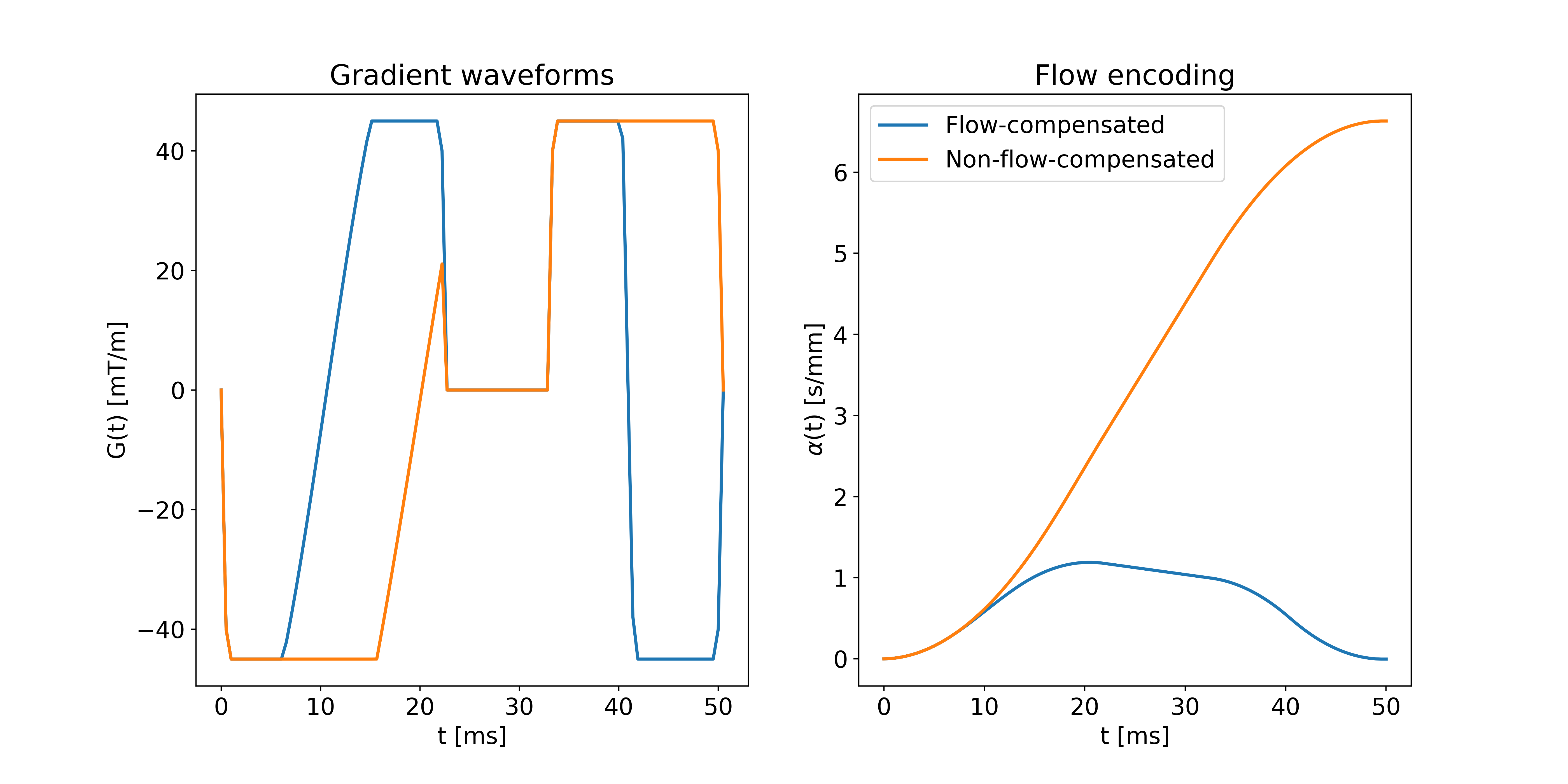
Generation of gradient waveforms
Flow-compensated and non-flow-compensated gradients waveforms were obtained through numerical optimization⁵. For a given encoding time $$$T$$$, the optimization maximized $$$b$$$ given the constraints: maximum gradient strength 45mT/m, maximum slew rate 100T/m/s, minimal influence of concomitant fields⁶, and zero gradient at endpoints and during the refocusing RF pulse (10ms). To account for the start of the EPI readout, the time available for the gradient waveform was 5ms shorter after the refocusing RF pulse than before. To achieve flow-compensation, the flow-encoding strength ($$$\alpha$$$) was constrained to be zero at $$$t=T$$$, with:$${\bf{\alpha}}=-\int_0^T{\bf{q}}(t)dt$$$${\bf{q}}(t)=\gamma\int_0^t{\bf{G}}(t')dt'$$where $$$\gamma$$$ is the gyromagnetic ratio and $$$G(t')$$$ is the gradient waveform³. Gradient waveforms were generated with and without flow-compensation for encoding times 30,50,70,90ms. An example ($$$T=50$$$ms) is shown in Figure 1.

Calculation of $$$F_P$$$
Following Wetscherek², the signal attenuation of the perfusion compartment for a given gradient waveform was assumed to be given by:$$F_P=\int{P({\bf{v}}|l)e^{i\phi({\bf{v}},l)}d{\bf{v}}}=\iint{P(v,\varphi|l)e^{ivG\varphi(v,l)}dvd\varphi}=\int{P(v)}\int{P(\varphi|v,l)e^{ivG\varphi(v,l)}d{\varphi}dv}$$$$\phi({\bf{v}},l)=\int_0^T{\bf{v}}(t;l)\cdot{\bf{q}}(t)dt=vG\varphi(v,l)$$$$$\varphi$$$ thus only depends on $$${\bf{q}}_{norm}(t)={\bf{q}}(t)/G$$$ and $$$N=T/\tau=Tv/l$$$.
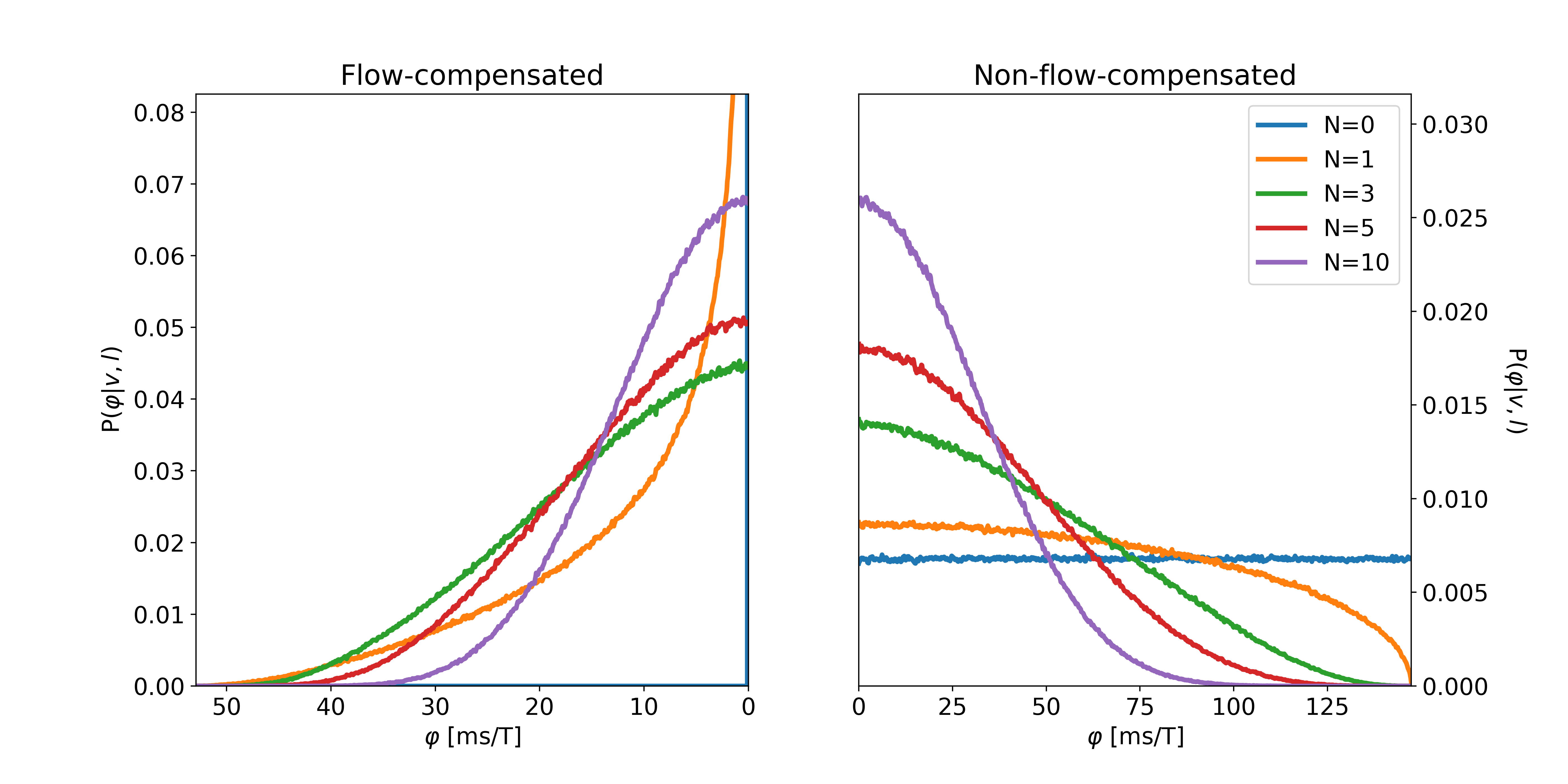
Normalized phase distributions $$$P(\varphi|v,l)$$$ were obtained via numerical simulations², where the normalized phase was calculated as:$$\varphi_j=\sum_{k=0}^{K-1}\hat{v}_j^{(k)}q_{norm}^{(k)}$$where $$$K$$$ is the number of time points, $$$q_{norm}^{(k)}$$$ represents the discretized gradient waveform, and $$$\hat{v}_j^{(k)}\sim\mathcal{U}(-1,1)$$$, enclosing both the spherically uniform distribution of $$$\bf{v}$$$ and the scalar product. $$$\hat{v}_j^{(k)}$$$ was regenerated when $$$k$$$ was a multiple of $$$\lfloor{r_j(K-1)/N}\rfloor$$$, where $$$r_j\sim\mathcal{U}(0,1)$$$ corresponds to the position of spin $$$j$$$ in the vessel segment at $$$t=0$$$.
For each gradient waveform, $$$P(\varphi|v,l)$$$ was generated based on 6,400,000 random walkers. Example distributions are shown in Figure 2.

In vivo data
A healthy volunteer was scanned on a Philips 3T Achieva dStream using a software patch enabling diffusion encoding with arbitrary gradient waveforms⁷. Diffusion-weighted images of the upper abdomen with b-values 0,10,20,30,40,50,75,100,125,150s/mm² were obtained using the flow-compensated and non-flow-compensated gradient waveforms with $$$T=50$$$ms. Other imaging parameter: TE=70ms, voxel size 3×3×5mm³. The study was approved by the regional ethical review board in Gothenburg, Sweden.
The average signal was extracted from a region of interest in the liver for further analysis. Models corresponding to the ballistic, intermediate and diffusive regimes were fitted to data, with predefined value for $$$v=5$$$mm/s and $$$\tau=150$$$ms from the literature^2,4.

Results & Discussion

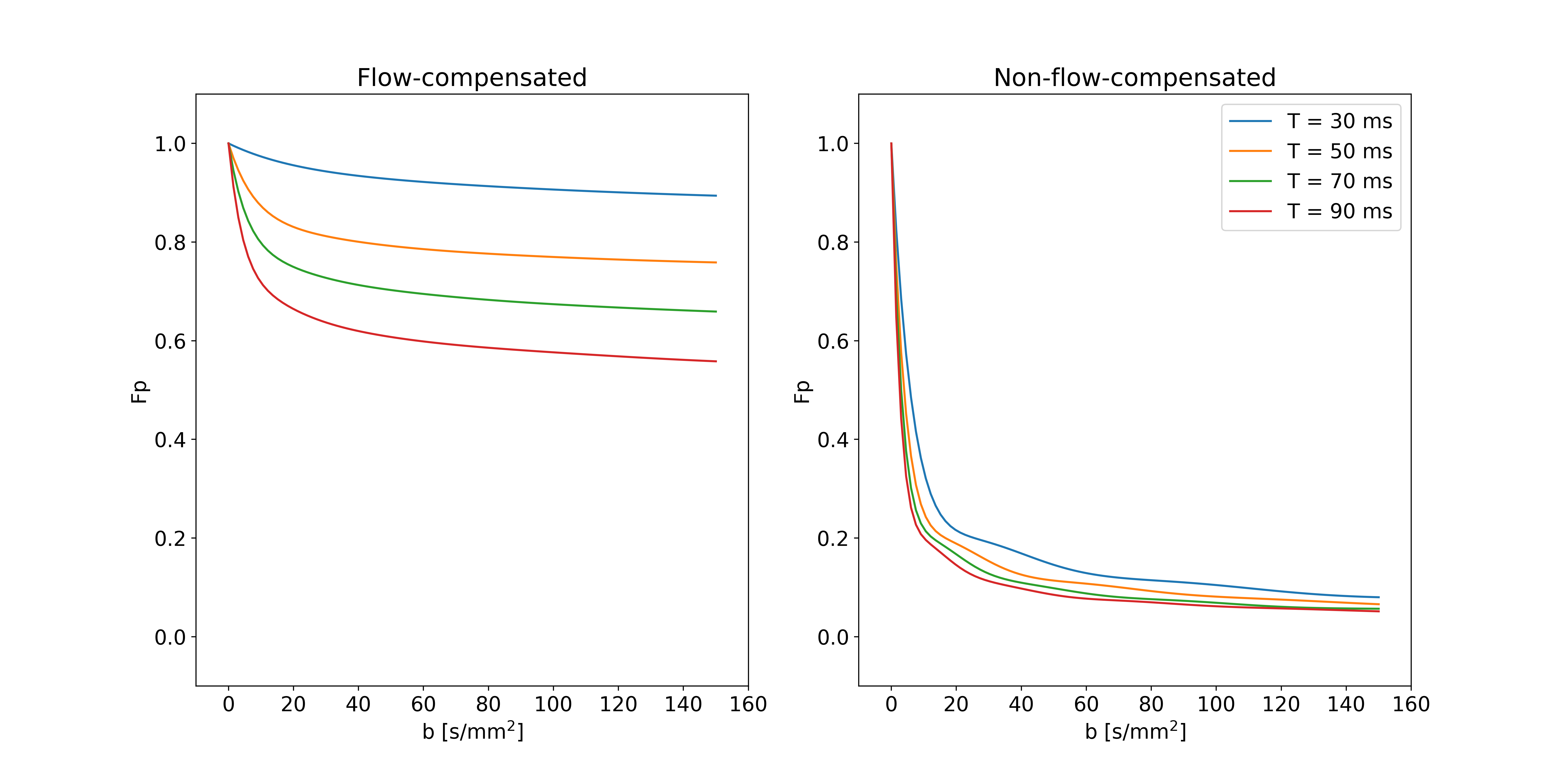
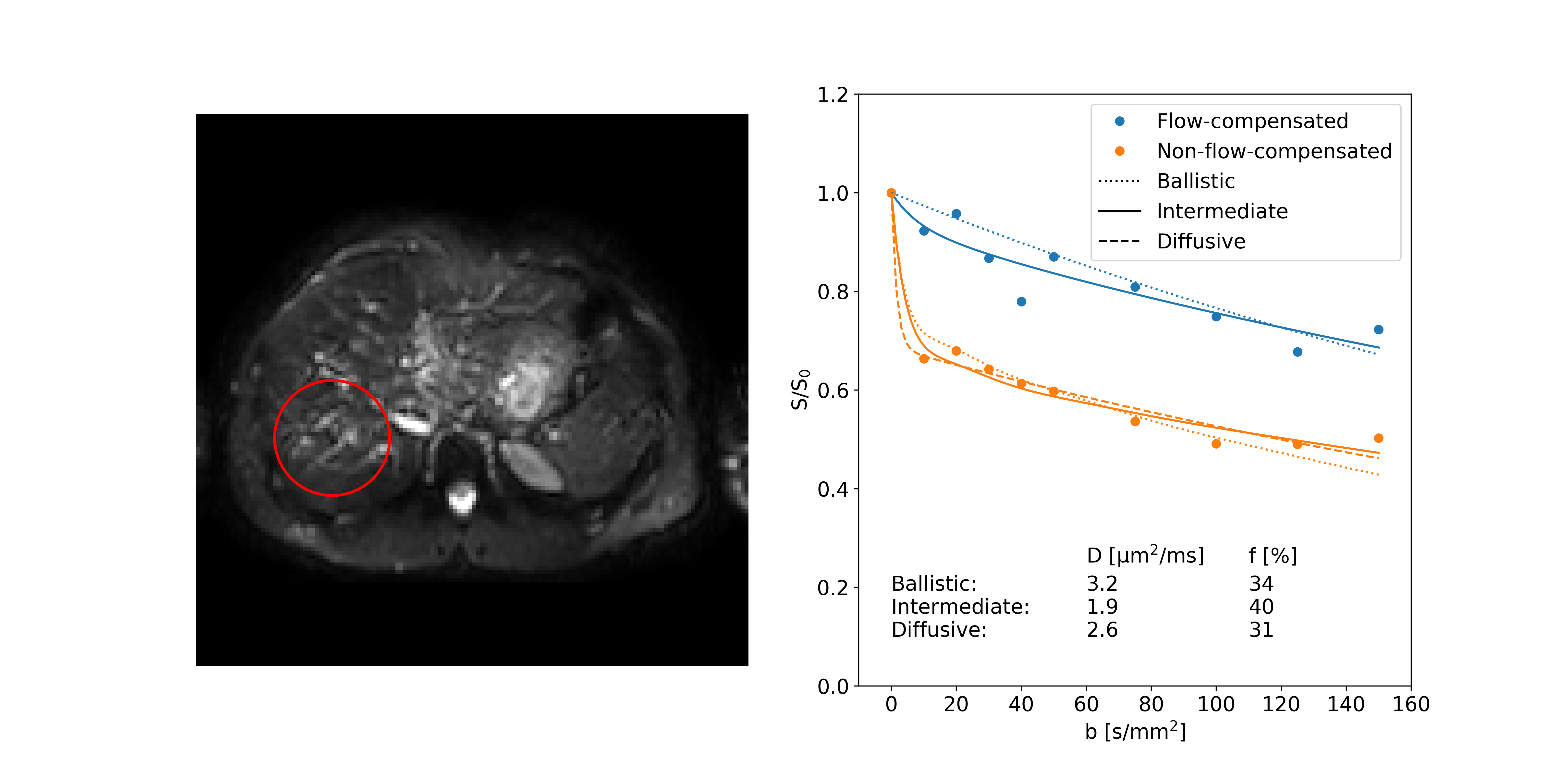
The encoding time had a substantial influence on $$$F_P$$$ when flow-compensated gradient waveforms were used (Fig. 3). Even at the shortest $$$T$$$, $$$F_P$$$ was far from the behavior predicted by the ballistic regime ($$$F_P=1$$$). In contrast, when non-flow-compensated gradient waveforms were used, $$$T$$$ had only minor effects, although it should be noted that $$$F_P$$$ did not go to zero as quickly as depicted by the diffusive regime.
A distinct signal difference between data using flow-compensated and non-flow-compensated gradient waveforms could be seen in the liver (Fig. 4). This agrees with previous studies^2,4,8 and further demonstrates the inappropriateness of assuming the diffusive regime for healthy liver tissue.
Among the model fits, the intermediate-regime model produced the best fit with residuals fairly randomly distributed around the model fit (Fig. 4). While the ballistic-regime model could capture most of the effect of flow-compensation, it did show structured residuals for the flow-compensated data, especially at low b-values, and also estimated an unrealistically large diffusion coefficient. The diffusive-regime model provided a good fit to the non-flow-compensated data, but is inherently unable to capture the signal difference introduced by flow-compensation seen in the current data.
The perfusion fraction estimated with the intermediate-regime model was substantially larger (≈25%) than what was given by the other two models, agreeing with what was expected from the results in Figure 3. Inaccurate modeling assumptions may thus have a significant influence on parameter estimates. The potential impact on results from previous and future studies on healthy liver and other tissue types should therefore be further studied.

Conclusion

The IVIM caused by microcirculation in the healthy liver appears to occur somewhere between the ballistic regime and the diffusive regime. Using any of the extreme regimes as a basis for modeling may introduce substantial bias to estimated parameters.

References

1. Le Bihan D, Breton E, Lallemand D, Aubin ML, Vignaud J, Laval-Jeantet M. Separation of diffusion and perfusion in intravoxel incoherent motion MR imaging. Radiology 1988;168:497–505.
2. Wetscherek A, Stieltjes B, Laun FB. Flow-compensated intravoxel incoherent motion diffusion imaging. Magn Reson Med 2015;74:410–419.
3. Ahlgren A, Knutsson L, Wirestam R, Nilsson M, Ståhlberg F, Topgaard D, Lasic S. Quantification of microcirculatory parameters by joint analysis of flow-compensated and non-flow-compensated intravoxel incoherent motion (IVIM) data. NMR Biomed 2016;29:640–649.
4. Gurney‐Champion OJ, Rauh SS, Harrington K, Oelfke U, Laun FB, Wetscherek A. Optimal acquisition scheme for flow‐compensated intravoxel incoherent motion diffusion‐weighted imaging in the abdomen: An accurate and precise clinically feasible protocol. Magn Reson Med 2019 In press.
5. Sjölund J, Szczepankiewicz F, Nilsson M, Topgaard D, Westin C-F, Knutsson H. Constrained optimization of gradient waveforms for generalized diffusion encoding. J Magn Reson 2015;261:157–168.
6. Szczepankiewicz F, Nilsson M. Maxwell-compensated waveform design for asymmetric diffusion encoding. Proc Jt Annu Meet ISMRM-ESMRMB, Paris, Fr 2018;100:207.
7. Westin C-F, Knutsson H, Pasternak O, et al. Q-space trajectory imaging for multidimensional diffusion MRI of the human brain. Neuroimage 2016;135:345–362.
8. Moulin K, Aliotta E, Ennis DB. Effect of flow-encoding
strength on intravoxel incoherent motion in the liver. Magn Reson Med 2018;81:1521-1533.