4418
A New Method for Reconstructing the Orientation Distribution Function in HARDI1Center for Nano & Micro Mechanics, Tsinghua University, Beijing, China, 2Center for Biomedical Imaging Research, Department of Biomedical Engineering, School of Medicine, Tsinghua University, Beijing, China
Synopsis
We propose a novel definition of orientation distribution function (ODF), which also represents diffusion coefficients for non-Gaussian situations, thus ODF has physical meaning. Then an expression is derived to calculate ODF values through diffusion-weighted signals. Next a new HARDI (high angular resolution diffusion imaging) method called “g-OPDT” (grids orientation probability density transform) is designed for practical use. Numerical simulations are performed to verify its accuracy. ISMRM-2015-Tracto-challenge data are used to quantitatively compare g-OPDT with other methods. Results show that g-OPDT has superior performance on most indicators. In-vivo experiments are conducted to show that its glyph representations have less redundant lobes.
Introduction
High angular resolution diffusion imaging (HARDI) methods are powerful techniques to describe the neural architecture especially in a voxel which contains multiple fibers including crossing, bending, or kissing.1,2 Based on the probability density function (PDF) P(r), the orientation distribution function (ODF) is calculated to characterize the information about orientation. The following two ways are usually used,3-5$$ \Psi_{\text {tuch }}(\mathbf{u})=\int_{0}^{\infty} P(r \mathbf{u}) d r $$
$$\Phi_{\operatorname{marg}}(\mathbf{u})=\int_{0}^{\infty} P(r \mathbf{u}) r^{2} d r $$
Here Ψtuch(u) is defined as the radial integration of PDF, but its integral on the entire sphere is not 1; Φmarg(u) is a true PDF due to the inclusion of the Jacobian factor r2 in the integration. Several single-shell HARDI techniques3,5-7 are realized on them, and their ODFs are derived by the Funk-Radon Transform (FRT)16.
Here, we propose a new definition of ODF as follows,
$$\Psi(\mathbf{u})=\int_{0}^{\infty} P(\mathbf{u} r) r d r$$
The expression to calculate Ψ(u) by diffusion-weighted signals is obtained through mathematical derivations. We show that it is also regarded as the diffusion coefficient for non-Gaussian situations. Instead of using FRT, a grid-algorithm is designed based on the proposed definition as a new estimator called “g-OPDT”. Then we compare the new estimator with other popular ones like OPDT,5,7 c-OPDT,6,7 p-OPDT6 on simulation experiments, ISMRM-2015-Tracto-challenge data17 and real HARDI datasets to show the superiority of g-OPDT.
Theory
For anisotropic Gaussian diffusion8:$$$P(\mathbf{u} r)=\frac{1}{(4 \pi \tau)^{1.5}|\mathbf{D}|^{0.5}} \exp \left(-r^{2} \mathbf{u}^{\mathrm{T}} \mathbf{D}^{-1} \mathbf{u}\right)$$$, where D is the diffusion tensor and uTDu represents the diffusion coefficient along u. Note that 1/ uTD-1u has the same unit as uTDu and also describes the diffusion coefficient.For non-Gaussian diffusion, the Gaussian model can be generalized to:
$$P(\mathbf{u} r)=\frac{1}{Z} \exp \left(-r^{2} \varphi(\mathbf{u})\right)$$
where Z is a normalization factor and φ(u) is an orientation function defined on the unit sphere, which describes the diffusion movement along u and equals to uTD-1u for Gaussian diffusion. According to the new ODF, we have:
$$\Psi(\mathbf{u})=\int_{0}^{\infty} P(\mathbf{u} r) r d r=\frac{1}{2 Z} \varphi(\mathbf{u})^{-1} \propto \frac{1}{\varphi(\mathbf{u})}$$
For Gaussian diffusion, 1/φ(u) equals to 1/uTD-1u. Similarly, for non-Gaussian situations,1/φ(u) also represents diffusion coefficients, which means the new definition of ODF has a clear physical meaning. According to radial mono-exponential model,8,9 Ψ(u) is calculated by diffusion-weighted signals and its grid-algorithm is :
$$\Psi(\mathbf{u})=\frac{1}{2 \sqrt{\pi} \sqrt{a(\mathbf{u})}}-\frac{1}{2 \pi^{1.5}} \sum \frac{1}{\sin 2 \theta} \frac{\partial}{\partial \theta}\left(\frac{1}{\sqrt{a(\theta, \varphi)}}\right) \Delta S-\frac{\theta_{0}}{2 \pi^{1.5}} \sum \frac{\partial^{2}}{\partial \theta^{2}}\left(\frac{1}{\sqrt{a(\theta, \varphi)}}\right)_{\theta=0} \Delta \varphi$$
Where $$$a(\theta, \varphi)=-\ln (E(\theta, \varphi))$$$,and the corresponding auxiliary coordinate system (θ,φ) is shown in the Fig. 1.The above reconstruction method for Ψ(u) is named as “g-OPDT’, where “g” represents “grids”.
Validations and Results
Simulations: Numerical validation is performed on artificial data generated by a two-tensor model,6,10 which is shown as:$$\mathrm{E}(\mathbf{u})=0.5\left(\exp \left(-\mathbf{u}^{\mathrm{T}} \cdot b \cdot \mathbf{D}_{1} \cdot \mathbf{u}\right)+\exp \left(-\mathbf{u}^{\mathrm{T}} \cdot \mathbf{b} \cdot \mathbf{D}_{2} \cdot \mathbf{u}\right)\right)$$
Fig. 2 shows the angle errors in resolving two crossing fibers by different estimators. For high b-values (b≥3000 sec/mm2), g-OPDT shows a relatively better trade-off between resolution and accuracy. Its angle errors are the smallest for large crossing angles while its resolution can also be maintained.
Fig. 3 shows the comparisons of different estimators in the presence of noise . For the low noise condition, i.e. SNR=50, g-OPDT basically maintains the same resolution as the noiseless case (Fig. 2). For SNR=20, its behavior is almost the same as others except for q-ball imaging (QBI).
ISMRM-2015-Tracto-challenge data: The challenge provides a simulated replication of whole brain diffusion data and creates a ground-truth for scoring. We reconstruct ODFs in each voxel by four estimators: OPDT, c-OPDT, p-OPDT and g-OPDT. All other operations, raw data pre-processing, seed points selecting, deterministic tractography and post-processing, remain the same. The scoring system provides five indicators as overall scores18 to quantitatively evaluate the imaging results. Local scores19 are calculated to evaluate their performance on partial regions and bundles. Fig. 4 lists overall and local scores of different estimators. Through Hypothesis Test,11,12 it is statistically convincible that g-OPDT performs best.
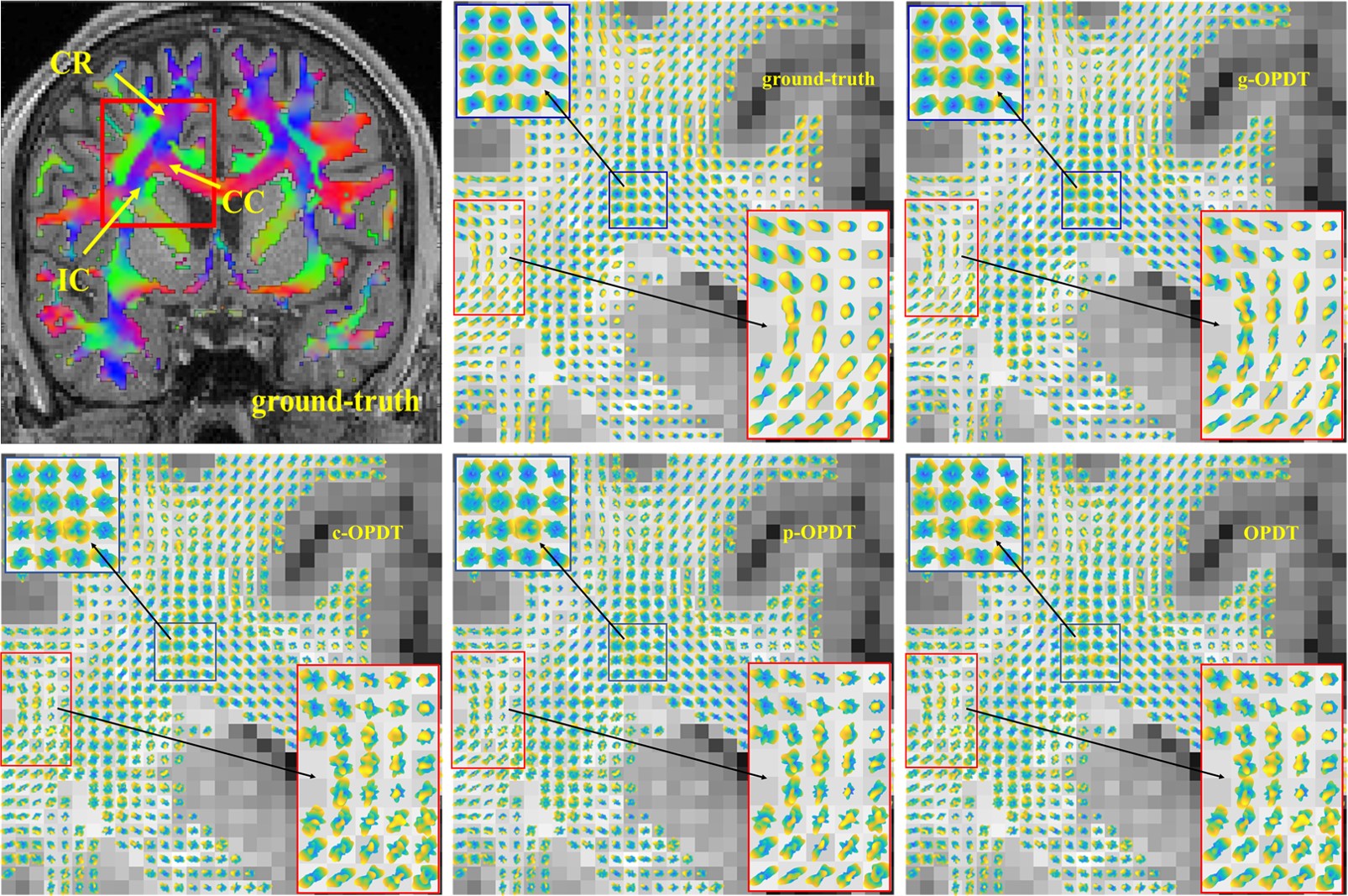
In vivo datasets: We downloaded three datasets generated by Human Connectome Project13-15 (HCP) to compare the performance of above estimators. They comprise 18 non-weighted baseline images and 270 diffusion encoding directions, which are distributed on three shells with b=1000,2000 and 3000 sec/mm2 (90 gradient directions on each shell), and their sizes are 145×174×145. The QBI method is used to reconstruct ODFs from the full data sampled in 270 directions. Its result is considered as the ground-truth to compare with other ones from down-sampled data (90 directions with b=1000 sec/mm2). Fig. 5 shows glyph representations of estimators in the Region of Interest (ROI) to illustrate the superiority of g-OPDT. The fibers show a local sharp bend in the red ROI in g-OPDT, consistent with those of the ground truth. The redundant lobes in the results of other OPDT-based methods blur the fiber orientation and break the spatial continuity of the glyphs.
Discussion and Conclusion
The new method performs well on different validations. The superiority of g-OPDT is evident on real human brain data, because the grid-algorithm effectively eliminates partial effects of noise compared to FRT. The less spurious lobes in the glyphs of g-OPDT confirm our conclusion and its reliability in vivo data.Acknowledgements
References
1. Tuch DS, Reese TG, Wiegell MR, Makris N, Belliveau JW, Wedeen VJ. High angular resolution diffusion imaging reveals intravoxel white matter fiber heterogeneity. Magn Reson Med 2002;48(4):577-582.
2. Tuch DS, Reese TG, Wiegell MR, Wedeen VJ. Diffusion MRI of complex neural architecture. Neuron 2003;40(5):885-895.
3. Tuch DS. Q-Ball imaging. Magn Reson Med 2004;52(6):1358-1372.
4. Aganj I, Lenglet C, Sapiro G. Odf Reconstruction in Q-Ball Imaging with Solid Angle Consideration. 2009 Ieee International Symposium on Biomedical Imaging: From Nano to Macro, Vols 1 and 2 2009:1398-1401.
5. Tristan-Vega A, Westin CF, Aja-Fernandez S. Estimation of fiber Orientation Probability Density Functions in High Angular Resolution Diffusion Imaging. Neuroimage 2009;47(2):638-650.
6. Aganj I, Lenglet C, Sapiro G, Yacoub E, Ugurbil K, Harel N. Reconstruction of the Orientation Distribution Function in Single- and Multiple-Shell q-Ball Imaging Within Constant Solid Angle. Magn Reson Med 2010;64(2):554-566.
7. Tristan-Vega A, Westin CF, Aja-Fernandez S. A new methodology for the estimation of fiber populations in the white matter of the brain with the Funk-Radon transform. Neuroimage 2010;49(2):1301-1315.
8. Basser PJ, Mattiello J, Lebihan D. Estimation of the Effective Self-Diffusion Tensor from the Nmr Spin-Echo. J Magn Reson Ser B 1994;103(3):247-254.
9. Stejskal EO, Tanner JE. Spin Diffusion Measurements: Spin Echoes in the Presence of a Time-Dependent Field Gradient. J Chem Phys 1965;42(1):288-292.
10. Tristan-Vega A, Westin CF. Probabilistic ODF Estimation from Reduced HARDI Data with Sparse Regularization. Medical Image Computing and Computer-Assisted Intervention (Miccai 2011), Pt Ii 2011;6892:182-190.
11. Neyman J. On the problem of the most efficient tests of statistical hypotheses. Philos T R Soc Lond 1933;231:289-337.
12. Berkson J. Tests of significance considered as evidence. J Am Stat Assoc 1942;37(219):325-335.
13. Setsompop K, Kimmlingen R, Eberlein E, et al. Pushing the limits of in vivo diffusion MRI for the Human Connectome Project. Neuroimage 2013;80:220-233.
14. McNab JA, Edlow BL, Witzel T, et al. The Human Connectome Project and beyond: Initial applications of 300 mT/m gradients. Neuroimage 2013;80:234-245.
15. Fan QY, Witzel T, Nummenmaa A, et al. MGH-USC Human Connectome Project datasets with ultra-high b-value diffusion MRI. Neuroimage 2016;124:1108-1114.
16. Funk P. Über eine geometrische Anwendung der Abelschen Integralgleichnung. Math Ann 1916; 77,129–135.
17. http://tractometer.org/ismrm_2015_challenge/data
18. http://tractometer.org/ismrm_2015_challenge/evaluation
19. http://tractometer.org/ismrm_2015_challenge/tools
Figures
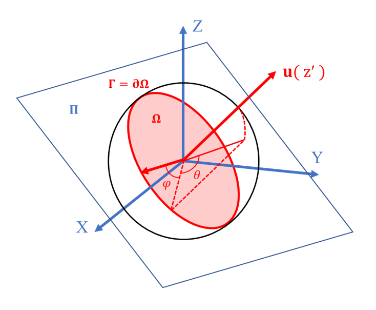
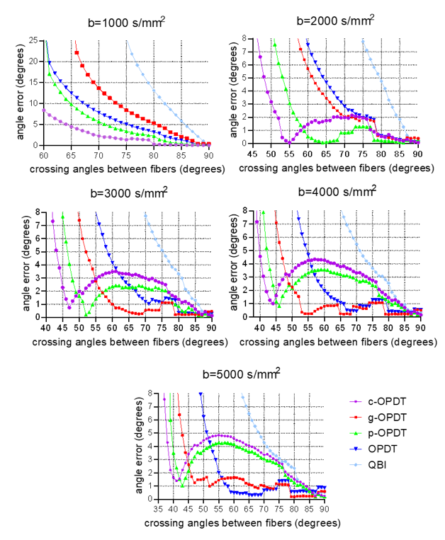
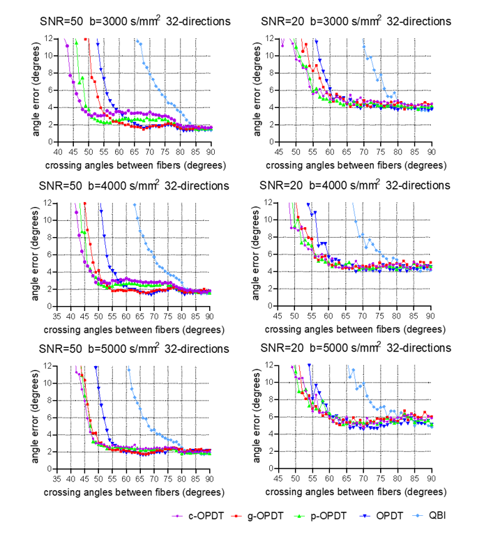
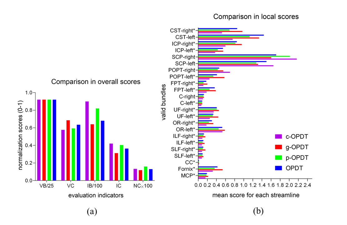
Fig. 4. Comparisons on ISMRM-challenge data. (a) Comparison in overall scores. VB: the number of valid bundles (≤ 25). VC: the percentage of streamlines that are part of the valid bundles. IB: the number of bundles that seem realistic but are not valid bundles. IC: the percentage of streamlines that are part of the invalid bundles. NC: the percentage of streamlines that are not assigned to VC or IC. (b) Comparison in local scores, which represent the mean score of streamlines on each ground-truth bundle. The local score of g-OPDT is the highest on the valid bundle whose name is labeled by “*”.