Introduction

Multi-dimensional magnetic resonance imaging (MRI) techniques have been proposed to investigate more specific information about the microstructure of biological tissue. A standard analysis technique is to estimate the joint probability distribution function of T1, T2 relaxation and diffusion coefficients, by solving an inverse Laplacian transform^[1-7]. But this approach is quite ill-posed and usually requires a large number of data points with strong regularization constraints to ensure reliable estimation. To overcome this limitation, we introduced an approach in [8] to estimate the moments of the joint probability distribution using the cumulant expansion of signal model. While [8] was focused on the joint moments of T2 relaxation and diffusion coefficients, this framework can be extended to more dimensions. In this work, we introduce the expressions for estimating the joint moments of T1 relaxation, T2 relaxation and diffusion coefficients (corresponding to the 3-dimensional joint distribution of these quantities) with data acquired using inversion-recovery spin echo sequences.

Method

The MRI signal acquired using an inversion-recovery diffusion encoded spin echo sequence can be represented by the following model:
$$S({\rm TE},{\rm TI},b,{\bf u}) = S_0 \bigg|\int (1-2 e^{-{\rm TI} r_1}+e^{-{\rm TR} r_1})e^{-{\rm TE} r_2 -bD({\bf u})}\rho(r_1,r_2,D,{\bf u})) d r_1 d r_2 d D\bigg|,$$
where TE, TI, TR represents the echo time, inversion recovery time, and repetition time, respectively, and u represents the gradient direction of a single-pulse diffusion encoding sequence with b being the b-value, S₀ represents the proton density and |.| is the absolute value. Moreover, r₁ = 1/T₁, r₂= 1/T₂ are the T₁ and T₂ relaxation coefficients and D represents the diffusion coefficient of protons in the tissue. $$$\rho$$$ represents the joint probability distribution function of r₁, r₂ and D along the direction u. We assume that TR is fixed in the experiments. Following [8], the signal model can be approximated by the following cumulant expansion:
$$ \begin{align}
S({\rm TE},{\rm TI},b,{\bf u}) \approx &S_0 \bigg|\exp\left(-{\rm TE}r_2-bD({\bf u})+\tfrac12 [{\rm TE}~ b ]\left[\begin{matrix} \sigma_{r_2r_2}& \sigma_{r_2D}(\bf u)\\\sigma_{r_2D}({\bf u}) & \sigma_{DD}({\bf u}) \end{matrix}\right]\left[\begin{matrix} {\rm TE}\\ b \end{matrix}\right]\right)\\ &-2 \exp\left(-{\rm TI}r_1-{\rm TE}r_2-bD({\bf u})+\tfrac12 [{\rm TI~ TE}~ b ]\left[\begin{matrix} \sigma_{r_1r_1}& \sigma_{r_1r_2}& \sigma_{r_1D}({\bf u})\\ \sigma_{r_1r_2}&\sigma_{r_2r_2}& \sigma_{r_2D}(\bf u)\\\sigma_{r_1D}({\bf u})& \sigma_{r_2D}({\bf u}) & \sigma_{DD}({\bf u}) \end{matrix}\right]\left[\begin{matrix}{\rm TI}\\ {\rm TE}\\ b \end{matrix}\right]\right)\\ &+\exp\left(-{\rm TR}r_1-{\rm TE}r_2-bD({\bf u})+\tfrac12 [{\rm TR~ TE}~ b ]\left[\begin{matrix} \sigma_{r_1r_1}& \sigma_{r_1r_2}& \sigma_{r_1D}({\bf u})\\ \sigma_{r_1r_2}&\sigma_{r_2r_2}& \sigma_{r_2D}(\bf u)\\\sigma_{r_1D}({\bf u})& \sigma_{r_2D}({\bf u}) & \sigma_{DD}({\bf u}) \end{matrix}\right]\left[\begin{matrix}{\rm TR}\\ {\rm TE}\\ b \end{matrix}\right]\right)\bigg|.
\end{align}$$
Though this abstract only considers the second-order cumulant expansion, third-order models can be derived in a straightforward manner. The above expression can be simplified in several special scenarios. For example, if a fixed TE value is used to explore the coupling between r₁ and D, then the components involving r₂ can be ignored and the S0 can be replaced by the T₂-weighted signal . Moreover, if TR is fixed and is long enough such that exp(-TR r₁) is negligible, then the last exponential function can be neglected. Futuremore, if both TI and TR are fixed and multiple pairs of b and TE are acquired, then the signal becomes a function of TE and b and the corresponding third-order cumulant expansion was considered in [8].

Experiment

We have applied the above cumulant expansion to analyze two datasets acquired using different protocols. The first dataset was acquired using a prototype inversion-recovery spin-echo sequence with the following parameters: TI = 200, 500, 1000 ms, b=0, 200, 500, 1000, 2000, 3500 s/mm2 and TE=74 ms, TR=3330ms. Moreover, 20 unique diffusion-encoding directions were sampled for each volume with non-zero b-values. To use the proposed method, the acquired data was fit using the spherical-ridgelet approach [10] to obtain 27 co-linear directions. The second dataset was provided from the public multi-dimensional diffusion MRI challenge data (MUDI) acquired using the ZEBRA sequence [9]. The full dataset consisted of 1344 volumes with acquisition parameters: TE = 80, 105, 130 ms, b=0, 500, 1000, 2000, 3000 s/mm2, TI from 20 to 7323 ms. To apply the proposed approach, this dataset was resampled using spherical-ridgelet functions to obtain 27 co-linear directions at b=1000, 2000, 3000 s/mm2 and TI = 400, 1000, 1600 and 2200 ms.

Results

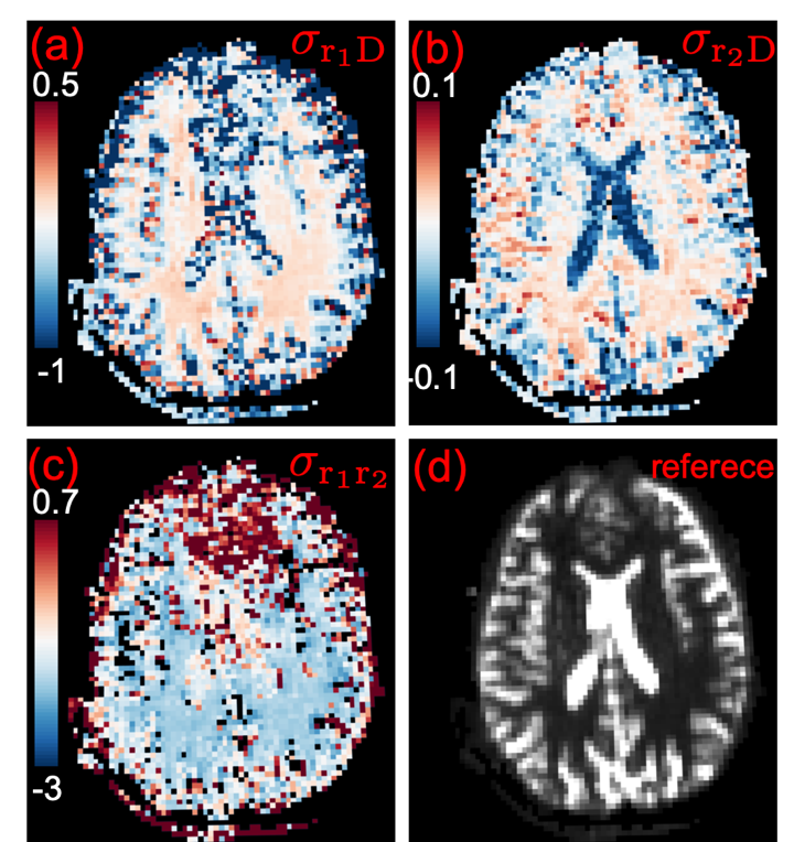
Figure (1a) illustrates the average cross covariance $$$\sigma_{r_1D}$$$ over all gradient directions for dataset 1. For completeness, Figure (1b) illustrates the $$$\sigma_{r_2D}$$$ map based on results from [8]. These maps show contrast between gray and white matters and contrast within white matters.

Figures(2a-2b) show the estimated $$$\sigma_{r_1D}$$$ and $$$\sigma_{r_2D}$$$ maps from dataset 2 for a slice shown in Figure (2d). The figures have similar contrast as the results shown in Figure 1.
Figure (2c) shows the cross-covariance $$$\sigma_{r_1r_2}$$$ between r₁ and r₂. The white matter shows negative correlations and the frontal-lobe gray matter shows relative strong positive correlations.

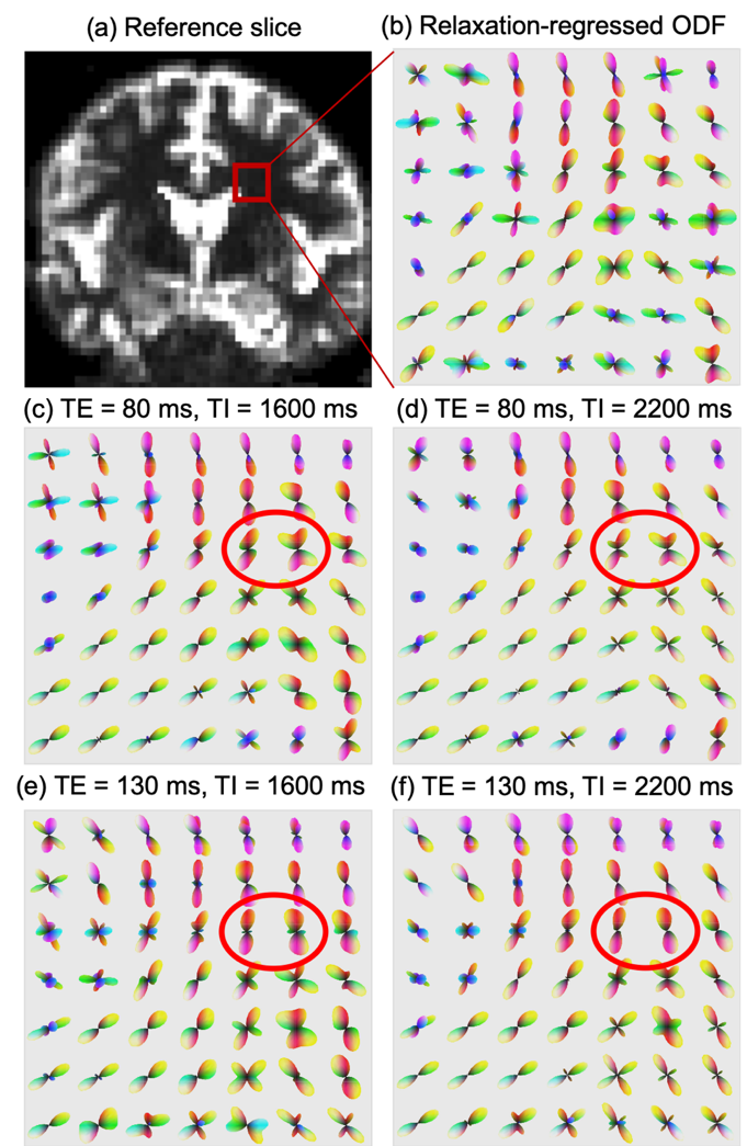
Figures (3c-3f) illustrate the fiber-orientation-distribution function for voxels in a brain region shown in Figure (3a). The ODF changes with varying TE and TI values indicating the underlying fiber bundles possibly have different relaxation coefficients. Figure (3b) shows the relaxation-regressed ODF estimated based on the mean and variance of diffusion coefficients.

Discussion and conclusions

The joint moment of multi-dimensional imaging parameters have shown promising new features to investigate tissue microstructure. But these parameters need to be validated using more datasets against histology, which will form part of our future work.

Acknowledgements

This work is supported in part by NIH grants R21MH116352, R21MH115280, K01MH117346, R01MH116173, R01MH111917, R01MH074794, P41EB015902.