Introduction

Free-water elimination (FWE) and mapping has been proposed to reduce the bias in DTI metrics induced by the partial-volume effect with free water.^1,2 FWE has been shown to be sensitive to the excess fluid in vasogenic oedema in human brain tumours.^1,2 Unfortunately, the FWE parameter estimation problem is ill-conditioned.^1,3 However, it has been demonstrated that the addition of a second dimension, spanned by the transverse relaxation time weighting, T₂ (FWET₂), mitigates the ill-conditioned problem.^4,5
It has been suggested that the pseudo-normalisation of DTI parameters, starting around 24 hours after stroke onset, is mainly due to the formation of vasogenic oedema.^6,7 The aim of this study is to investigate the spatiotemporal evolution of ischemic areas in stroke middle cerebral artery occlusion (MCAo) animal models using FWET₂ and to evaluate its potential for the characterisation of tissue microstructure in the presence of vasogenic oedema.

Methods

Theory. The model we adopt here assumes that the diffusion MRI signal originates from two compartments with different transverse relaxation rates and diffusivities. In the slow-exchange limit it reads as⁴ $$S_\mathrm{FWET_2}(T_\mathrm{E},b,\mathbf{n})=S_0[f_\mathrm{w}e^{-T_\mathrm{E}/T_{2,\mathrm{w}}}e^{-bD_\mathrm{w}}+(1-f_\mathrm{w})e^{-T_\mathrm{E}/T_{2,\mathrm{t}}}e^{-b\mathbf{n}^\mathrm{T}\mathbf{D}_\mathrm{t}\mathbf{n}}]\;\;\;(1)$$ where $$$S_0$$$ is the proton density, $$$f_\mathrm{w}$$$, $$$T_{2,\mathrm{w}}$$$ and $$$D_\mathrm{w}$$$ are the fraction, transverse relaxation time and diffusion coefficient of the free-water compartment and $$$T_\mathrm{2,t}$$$ and $$$\mathbf{D}_\mathrm{t}$$$ are the transverse relaxation time diffusion tensor for the tissue compartment. The strength and direction of the diffusion weighting gradient are $$$b$$$ and $$$\mathbf{n}$$$, respectively, and $$$T_\mathrm{E}$$$ is the echo-time. We assume that the vasogenic oedema can be modelled by the isotropic, Gaussian compartment.^1,2

Animal model. Nine adult, male Sprague–Dawley rats, weighting 350-450 g, were used. All procedures were approved by the Animal Care and Use Committee, National Health Research Institutes, Taiwan. After the pre-stroke scans, rats underwent the MCAo for 90 minutes as described previously.¹² Three groups of animals were measured at the following time points: group1{pre,1h,23h,45h,23d} (3 animals); group 2 {pre,11h,33h,23d} (2 animals); group 3 {pre,1d,3d,4d,5d,6d,7d,10d} (4 animals) (h=hours; d=days).

MRI experiments. Experiments were performed on a home-integrated 3T whole-body MRI scanner including an ultra-high-strength gradient coil with a maximum strength of 675 mT/m.⁸ A custom-designed, single-loop transmit/receive surface coil was utilised. A Stejskal-Tanner, segmented EPI pulse sequence was implemented in-house. Experimental parameters were: T_E=50ms and 100ms; b-values(directions) = 0(16), 0.5(24) and 1.0(52) ms/µm²; diffusion gradient separation and duration, Δ=24ms and δ=3ms. Additionally, four more echo-times, T_E=70,90,110,130ms (8 repetitions) were acquired. Other parameters were voxel-size=0.26×0.26×13mm³; matrix-size=96×96×20; repetition-time, T_R=9s. A turbo spin-echo sequence was used to acquire structural images. Protocol parameters were: T_R=4s; T_E=68ms; voxel-size=0.13×0.13×1mm³; matrix-size=192×192×20.

Data analysis. Following denoising⁹ and EPI and eddy-current distortion correction,¹⁰ all datasets were analysed using conventional DTI with an explicit, monoexponential T₂ attenuation (DTIT₂), where the signal is given by: $$$S_\mathrm{DTIT_2}(T_\mathrm{E},b,\mathbf{n})=S_0e^{-T_\mathrm{E}/T_2}e^{-b\mathbf{n}^\mathrm{T}\mathbf{Dn}}$$$. DTIT₂ model parameters were estimated using the weighted-linear least-squares estimator. FWET₂ model parameters were then estimated using the non-linear least-squares estimator, with the DTIT₂ parameters as the initial guess. All estimations were performed using in-house Matlab scripts. Free water parameters were fixed to: $$$T_{2,\mathrm{w}} = 1.25\;\mathrm{s}$$$ and $$$D_\mathrm{w} = 3\;\mathrm{μm^2/ms}$$$.¹¹

Results and discussions

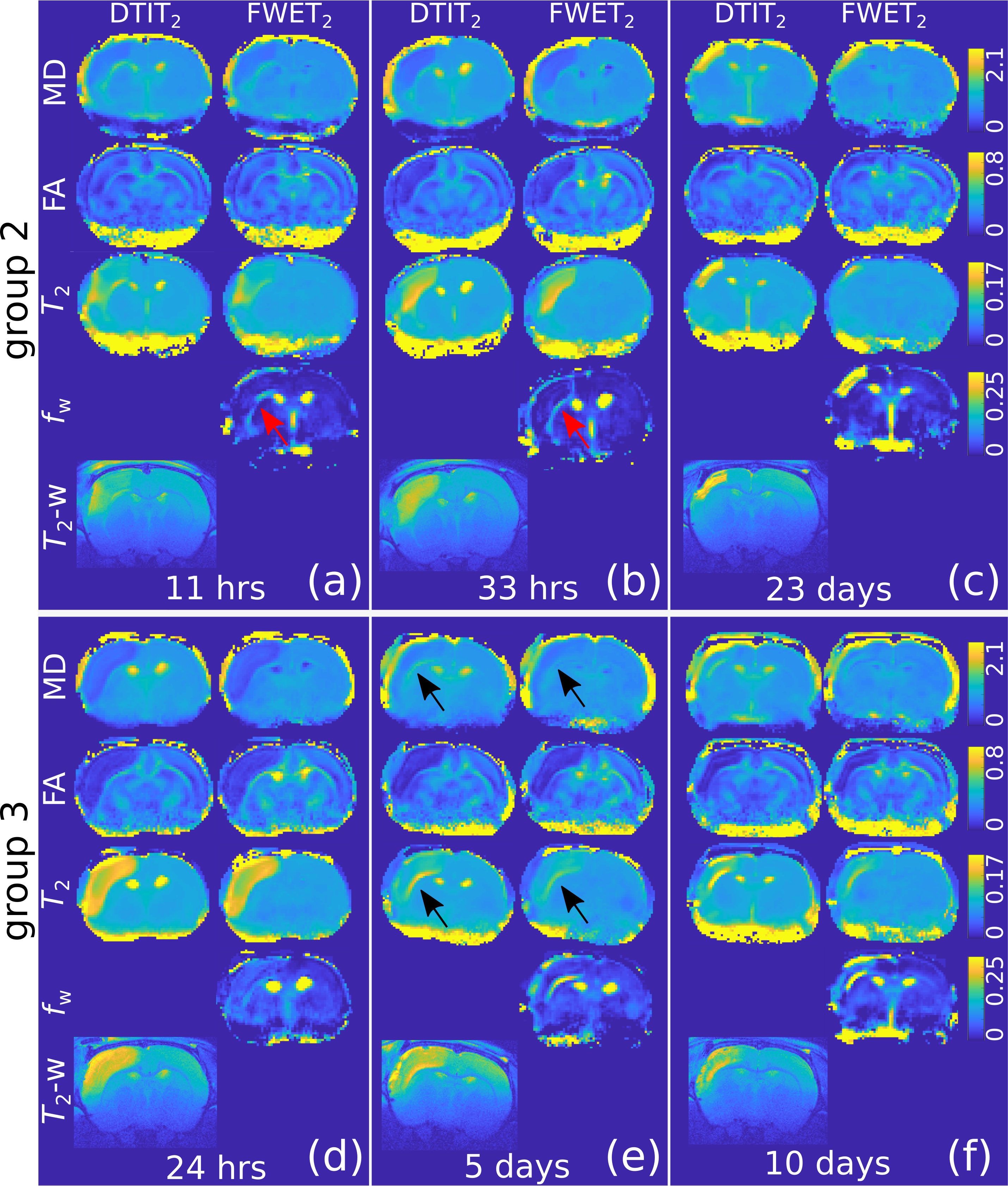
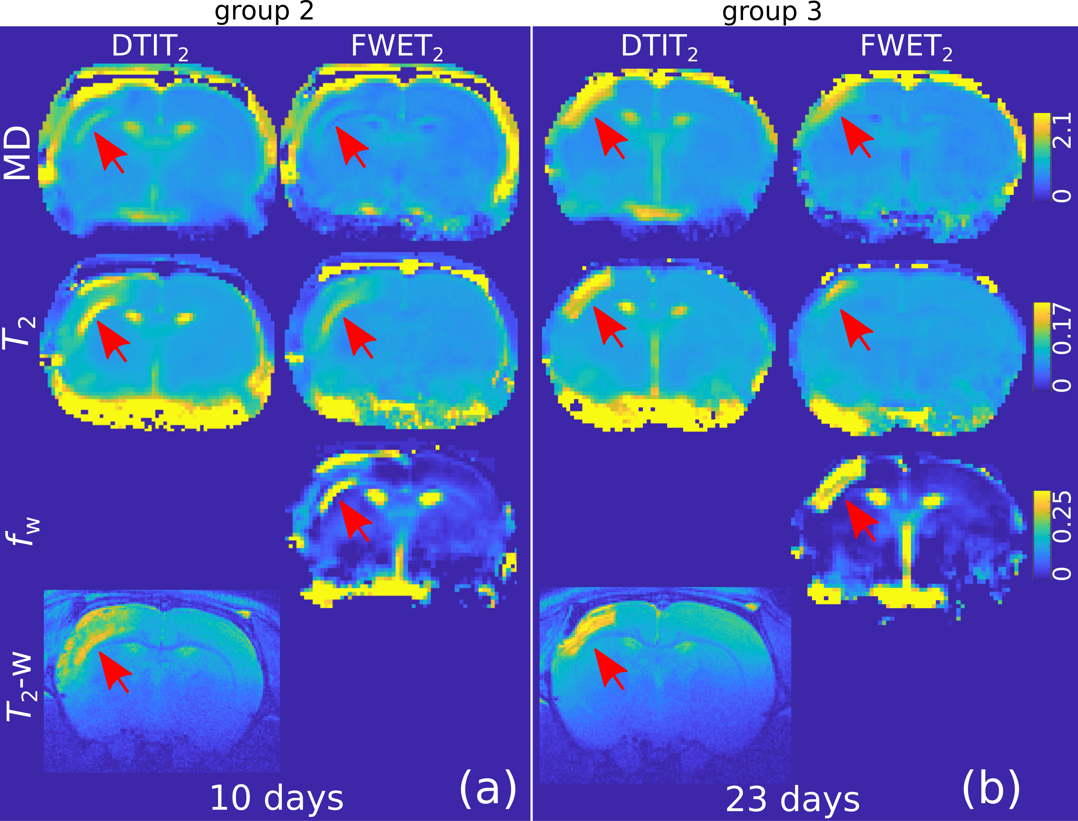
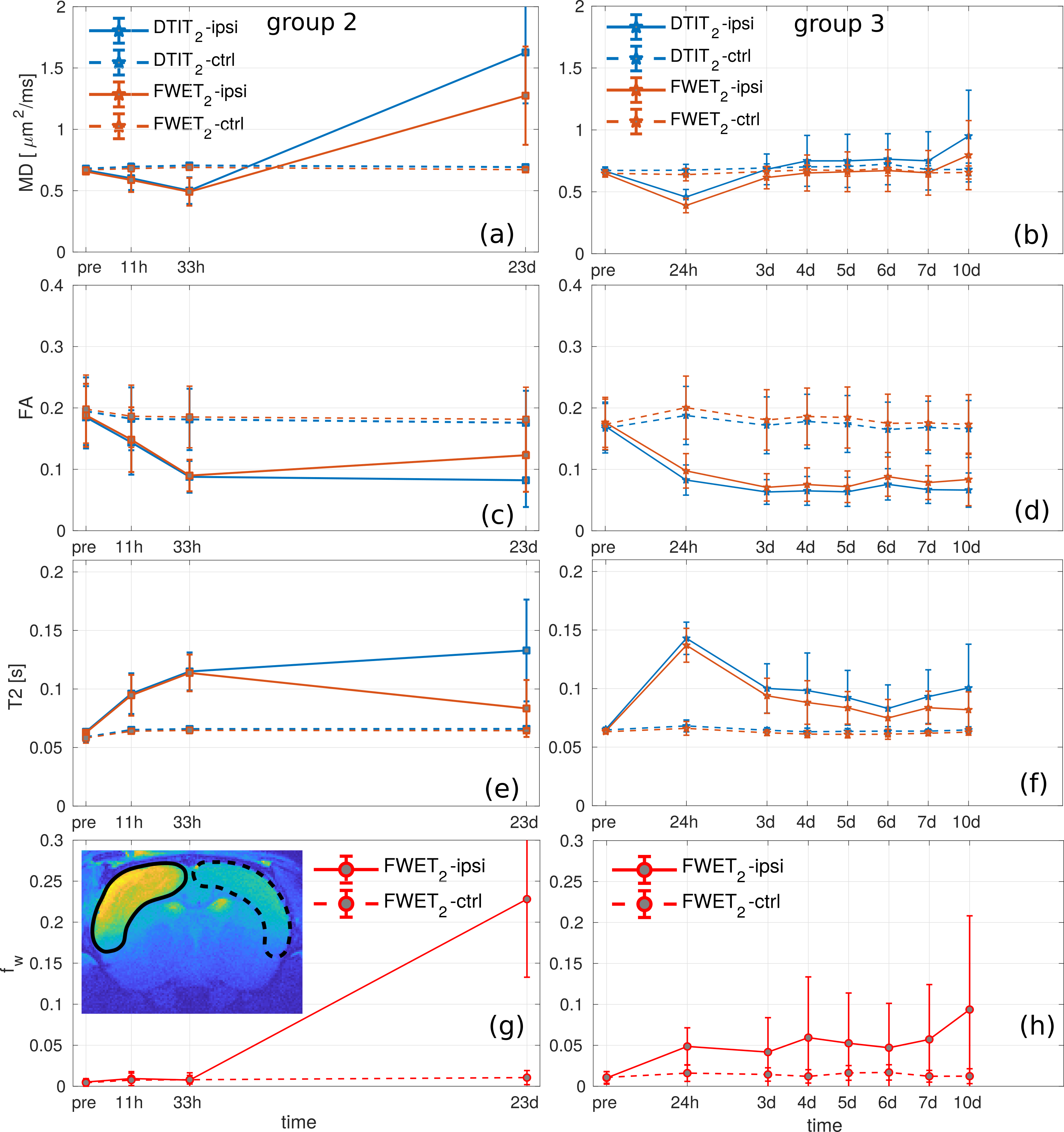
Fig. 1 shows DTIT₂ and FWET₂ maps for three selected time points for one representative animal from group 2 (a-c) and one representative animal from group 3 (d-f), as an example. A reduction of MD and FA, together with an increase in $$$T_2$$$, is observed up to 33 h after occlusion (Figs. 1a,b,d). Here, the difference between DTIT₂ and FWET₂ is minor, except for a slight increase in the free water fraction, $$$f_\mathrm{w}$$$, in the white matter (WM) at the ipsi-lateral side (red arrows, Figs.1a,b). At five days (Fig.1e) MD and $$$T_2$$$ tend to re-normalise (black arrows) and $$$f_\mathrm{w}$$$ in WM increases further. At 10 days (Fig.1f) MD and $$$T_2$$$ from DTIT₂ tend to increase. However, this is mostly due to the presence of excess fluid, which is reflected by the increase in $$$f_\mathrm{w}$$$ (zoomed maps, Fig.2a) and becomes more heterogeneous. At 23 days (Fig.1c), MD and $$$T_2$$$ from DTIT₂ show much higher values, which is reflected by the increase in $$$f_\mathrm{w}$$$ (red arrows, Fig.2b). MD and $$$T_2$$$ from FWET₂, which are not contaminated by free water, show much closer values to the contra-lateral side.
Fig. 3 shows the group-averaged temporal evolution of MD (a,b), FA (c,d), $$$T_2$$$ (e,f) and $$$f_\mathrm{w}$$$ (g,h) for both DTIT₂ (blue) and FWET₂ (red), for groups 2 (a,c,e,g) and 3 (b,d,f,h). During the acute phase, MD and FA are reduced and $$$T_2$$$ increases up to 33 hours after occlusion. Here the difference between DTIT₂ and FWET₂ is not significant. At three days, DTIT₂ parameters start showing increasing differences. These differences are partly reflected by the increase in $$$f_\mathrm{w}$$$ (Figs. 3g,h), leading to a reduction in MD and $$$T_2$$$ from FWET₂.

Conclusions

We demonstrated the application of FWET₂ for the investigation of the spatiotemporal evolution of ischemic lesions in MCAo stroke animal models. We found that, starting at nearly 3 days after stroke onset, the increase in excess fluid in the affected area induces changes in diffusion and relaxation parameters, which are reflected by the free water parameter, $$$f_\mathrm{w}$$$. Thus, FWET₂ is potentially helpful to investigate the evolution of vasogenic oedema and tissue-specific features, such as the ischemic penumbra and tissue heterogeneity during the chronic phase.

Acknowledgements

We thank Mrs Claire Rick for proof reading the manuscript.