4410
Trueness and precision of statistical descriptors obtained from multidimensional diffusion signal inversion algorithms1Physical Chemistry, Lund University, Lund, Sweden, 2Random Walk Imaging AB, Lund, Sweden, 3Physics, Università degli Studi di Milano, Milan, Italy
Synopsis
In first approximation, the diffusion signal writes as the Laplace transform of an intra-voxel diffusion tensor distribution (DTD). Several algorithms have been introduced to estimate the DTD’s statistical descriptors (mean diffusivity, variance of isotropic diffusivities, mean squared diffusion anisotropy, etc.) by inverting data obtained from tensor-valued diffusion encoding schemes. However, the trueness and precision of these estimations have not been systematically assessed and compared across methods. Here, we compare such estimations in silico for a 1D Gamma fit, a generalized two-term cumulant approach, and 2D and 4D Monte-Carlo inversion techniques, using a common and clinically feasible tensor-valued acquisition scheme.
Introduction
In biological tissues, typical MRI voxels comprise multiple microscopic environments, whose local organization can be captured by microscopic diffusion tensors. The measured diffusion MRI signal can, therefore, be written as the multidimensional Laplace transform of an intra-voxel diffusion tensor distribution (DTD).1 While tensor-valued diffusion encoding schemes have been designed to probe specific features of the DTD via the sizes (b-value $$$b$$$), shapes (normalized anisotropy $$$b_\Delta\in[-0.5,1]$$$) and orientations $$$(\Theta,\Phi)$$$ of encoding tensors $$$\mathbf{b}$$$,2-4 several algorithms have been introduced to invert such datasets and estimate statistical descriptors of the DTD. However, the trueness and precision of these estimations have not been systematically assessed and compared across inversion methods.Methods
We considered the estimations of three statistical descriptors:- the mean diffusivity $$$\mathrm{E}[D_\mathrm{iso}]$$$,
- the mean squared diffusion anisotropy $$$\tilde{\mathrm{E}}[D^2_\mathrm{aniso}]=\mathrm{E}[(D_\mathrm{iso}D_\Delta)^2]\,/\,\mathrm{E}[D_\mathrm{iso}]^2$$$,
- the variance of isotropic diffusivities $$$\mathrm{V}[D_\mathrm{iso}]$$$,
- 53 linearly encoded signals ($$$b_\Delta=1$$$) distributed as $$$6,10,16$$$ and $$$21$$$ points at $$$b=100,700,1400$$$ and $$$2000$$$ s/mm2, respectively.
- 32 spherically encoded signals ($$$b_\Delta=0$$$) sampled as $$$6,6,10$$$ and $$$10$$$ points at $$$b=100,700,1400$$$ and $$$2000$$$ s/mm2, respectively.
- one $$$b=0$$$ signal.
We compared the performances of four signal inversion techniques:
- for powder-averaged signals $$$\overline{\mathcal{S}}(b,b_\Delta)$$$, the Gamma fitting (Gamma)7 and the 2D Monte-Carlo inversion (MC-2D).8
- for non powder-averaged signals $$$\mathcal{S}(\mathbf{b})=\mathcal{S}(b,b_\Delta,\Theta,\Phi)$$$, the covariance tensor approximation (Cov, a tensorial two-term cumulant expansion)6 and the 4D Monte-Carlo inversion (MC-4D).9
To ensure fair comparison of the different inversion techniques, all readily available as Matlab code on GitHub,10,11 we follow these steps:
- A system is simulated by generating a set of ground-truth features $$$\{D_\mathrm{iso},D_\Delta,\theta,\phi,w\}$$$, from which the ground-truth descriptors and the ground-truth signals are computed using the general 4D kernel.
- Each signal inversion technique is run on an identical set of signals with added Rician noise at either signal-to-noise ratio (SNR) of 30 or at infinite SNR.
- Step 2 is repeated 100 times to build up statistics (medians and interquartile ranges) on estimation of the statistical descriptors.
Results and discussion
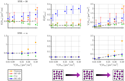
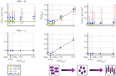
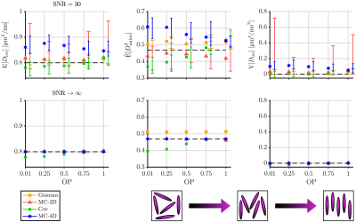
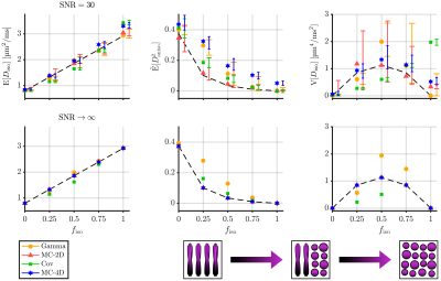
Figures 1, 2, 3 and 4 respectively present the effect of the variance of isotropic diffusivities, anisotropy, orientational order, and fraction of isotropic and anisotropic components on the descriptors' estimations for all investigated inversion methods.We found that these methods all share similar precision (except for a lower precision of MC-2D) but differ in term of trueness. Gamma exhibits infinite-SNR biases when the signal strongly deviates from mono-exponentiality and is unaffected by orientational order. As for Cov, it shows infinite-SNR biases when this deviation originates either from the variance in isotropic diffusivities or from the low orientational order of anisotropic diffusion components, because signals from such distributions contain features that are not captured by a two-term cumulant expansion. MC-2D shows remarkable trueness in all studied systems. However, its trueness in systems that are anisotropic at the voxel scale drastically worsens if the acquisition scheme does not possess enough directions to yield a good rotational invariance of the powder-averaged signal. Finally, MC-4D presents no infinite-SNR bias but significantly suffers from noise in the data, while preserving contrast in finite-anisotropy systems.
Conclusion
Methods that constrain the inversion (Gamma and Cov) exhibit, within the common acquisition scheme we chose, inherent limitations in estimating statistical descriptors, even at infinite SNR. Unconstrained methods (MC-2D and MC-4D) show perfect accuracy at infinite SNR but suffer from data noise, worsening either precision (MC-2D) or trueness (MC-4D) at finite SNR while preserving reasonable contrast. Future denoising efforts may alleviate these problems.Acknowledgements
This work was financially supported by the Swedish Foundation for Strategic Research (AM13-0090, ITM17-0267) and the Swedish Research Council (2018-03697). Daniel Topgaard owns shares in Random Walk Imaging AB (Lund, Sweden, http://www.rwi.se/), holding patents related to the described methods. We warmly thank Filip Szczepankiewicz and Markus Nilsson for fruitful discussions.References
1. Jian B, Vemuri BC, Özarslan E et al., A novel tensor distribution model for the diffusion-weighted MR signal. Neuroimage 2007;37(1):164-176.
2. Eriksson S, Lasic S and Topgaard D, Isotropic diffusion weighting in PGSE NMR by magic-angle spinning of the q-vector. Journal of Magnetic Resonance 2013;226:13-18.
3. Eriksson S , Lasic S, Nilsson M et al., NMR diffusion-encoding with axial symmetry and variable anisotropy: Distinguishing between prolate and oblate microscopic diffusion tensors with unknown orientation distribution. The Journal of Chemical Physics 2015;142(10):104201.
4. Topgaard D, Multidimensional diffusion MRI. Journal of Magnetic Resonance 2017; 275:98-113.
5. Szczepankiewicz F, Sjölund J, Ståhlberg F et al. Tensor-valued diffusion encoding for diffusional variance decomposition (DIVIDE): Technical feasibility in clinical MRI systems. PLOS ONE 2019;14(3):1-20.
6. Westin C-F, Knutsson H, Pasternak O et al. Q-space trajectory imaging for multidimensional diffusion MRI of the human brain. NeuroImage 2016;135:345-362.
7. Lasic S, Szczepankiewicz F, Eriksson S et al., Microanisotropy imaging: quantification of microscopic diffusion anisotropy and orientational order parameter by diffusion MRI with magic-angle spinning of the q-vector. Frontiers in Physics 2014;2:11.
8. de Almeida Martins J P and Topgaard D, Two-dimensional correlation of isotropic and directional diffusion using NMR. Physics Review Letters 2016;116:087601.
9. Topgaard D. Diffusion tensor distribution imaging. NMR in Biomedicine 2019;32(5):e4066
10. Nilsson M, Szczepankiewicz F, Lampinen B, et al. An open-source framework for analysis of multidimensional diffusion MRI data implemented in MATLAB. In: International Society for Magnetic Resonance Imaging (ISMRM) 2018.
11. Nilsson M, Szczepankiewicz F, C-F Westin and Topgaard D. MATLAB code for multidimensional diffusion MRI. https://github.com/daniel-topgaard/md-dmri. Accessed: 2019-07-09.
12. Reymbaut A, Gilbert G, Szczepankiewicz F et al., The “Magic DIAMOND" method: probing brain microstructure by combining b-tensor encoding and advanced diffusion compartment imaging. In: International Society for Magnetic Resonance Imaging (ISMRM) 2018.
Figures


